Hough transform
Faisal Qureshi
Professor
Faculty of Science
Ontario Tech University
Oshawa ON Canada
http://vclab.science.ontariotechu.ca
Copyright information
© Faisal Qureshi
License

This work is licensed under a Creative Commons Attribution-NonCommercial 4.0 International License.
Lesson Plan
- Hough transform
- Fitting lines to data
- Polar representation of a line
- Counting votes
- Applications
import numpy as np
import scipy as sp
import matplotlib.pyplot as plt
import matplotlib.lines as mlines
import matplotlib.cm as cm
from sklearn.cluster import KMeans
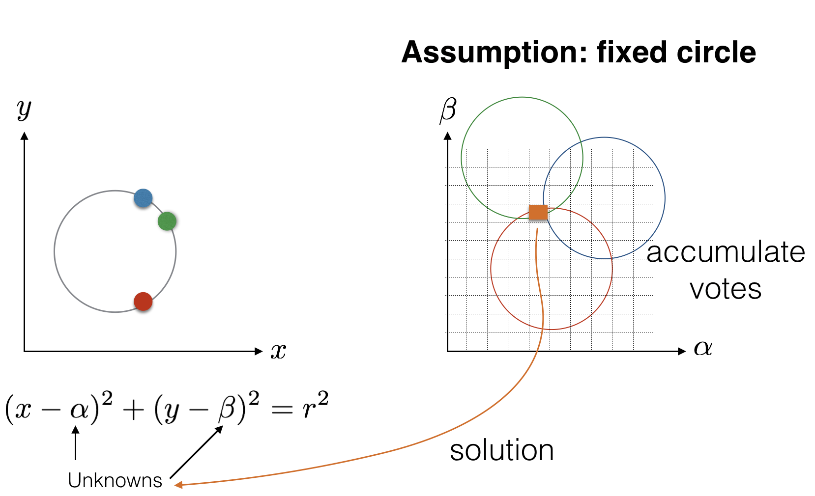
Hough transform
P.V.C. Hough, “Machine Analysis of Bubble Chamber Pictures,” Proc. Int. Conf. High Energy Accelerators and Instrumentation, 1959

Helper routines
Sampling points on a circle
def sample_circle(n=1, center=np.zeros(2), radius=1):
    """
    Returns an nx2 array
    """
    angles = np.random.rand(n)*2*np.pi
    pts = np.empty([2,n])

    for i in range(n):
        a = angles[i]
        r = np.array([np.cos(a), np.sin(a), -np.sin(a), np.cos(a)]).reshape(2,2)
        pts[:,i] = center + np.dot(r, np.array([radius,0]).reshape(2,1)).reshape(2)

    return pts.T
# x = sample_circle(10000, center=np.array([.5,.5]), radius=.3)
# plt.figure(figsize=(10,10))
# plt.plot(x[:,0], x[:,1], '.')
# plt.xlim(-2,2)
# plt.ylim(-2,2)
Line drawing
def draw_line(pt1, pt2, ax, **kwargs):
    """
    Draws a line passing through two points.
    """
    xmin, xmax = ax.get_xbound()
    ymin, ymax = ax.get_ybound()

    scale = np.sqrt((xmax - xmin)**2 + (ymax - ymin)**2)

    d = pt2 - pt1
    if np.isclose(np.linalg.norm(d), 0):
        print(f'draw_line warning:  pt1={pt1}, pt2={pt2}')

    s = pt1 - d * scale
    e = pt2 + d * scale

    l = mlines.Line2D([s[0], e[0]], [s[1], e[1]], **kwargs)
    ax.add_line(l)
def draw_line_mc(theta, ax, **kwargs):
    """
    Draws a line with slope m and y-intercept c
    """
    m = theta[0]
    c = theta[1]

    xmin, xmax = ax.get_xbound()

    ymin = m * xmin + c
    ymax = m * xmax + c

    l = mlines.Line2D([xmin, xmax], [ymin,ymax], **kwargs)
    ax.add_line(l)
def draw_line_polar(coord, ax, **kwargs):
    """
    Draws a line expressed in polar coordinates.  Here coord[0] is theta and coord[1] is rho.  Theta is in radians.
    """
    theta = coord[0]
    rho = coord[1]

    pt = np.array([
        rho * np.cos(theta),
        rho * np.sin(theta)
    ])

    n = pt / np.linalg.norm(pt)
    c = np.dot(n, pt)

    x2 = pt[0]+1
    y2 = (c - n[0]*x2) / n[1]

    return draw_line(pt, np.array([x2, y2]), ax, **kwargs)
# plt.figure(figsize=(10,10))
# draw_line(np.array([1,2]), np.array([1,2]), plt.gca())
# plt.xlim(-2,2)
# plt.ylim(-2,2)
def compute_m_and_c(pt1, pt2):
    A = np.array([pt1[0], 1, pt2[0], 1]).reshape(2,2)
    y = np.array([pt1[0], pt2[1]]).reshape(2,1)
    return np.dot(np.linalg.inv(A), y)
Hough transform
Lets generate some toy date to play with
def toy_data1():
    true_l1 = [1, 3]
    x1 = np.linspace(1,5,5)
    y1 = true_l1[0] * x1 + true_l1[1]

    true_l2 = [2, -5]
    x2 = np.linspace(5,7,3)
    y2 = true_l2[0] * x2 + true_l2[1]

    data = np.hstack([x1, x2, y1, y2]).reshape(2,-1).T
    return data, (0, 12, 0, 12)
Toy data
data, extents = toy_data1()
plt.figure(figsize=(7,7))
plt.title('Data')
plt.xlabel('x')
plt.ylabel('y')
plt.scatter(data[:,0], data[:,1], c='red')
plt.xlim(extents[:2])
plt.ylim(extents[-2:]);

The set of lines passing through a point
Lets pick a point and draw the set of lines that pass through them
id = 3

pt = data[id,:]
np.random.seed(0)
num_lines = 10
tmp = sample_circle(n=num_lines, center=pt, radius=1)
cmap = plt.get_cmap('Spectral')

mc = np.empty((num_lines, 2))
plt.figure(figsize=(7,7))
plt.title(f'Lines through pt=({pt[0]},{pt[1]})')
plt.xlabel('x')
plt.ylabel('y')
plt.scatter(data[:,0], data[:,1], c='blue', alpha=0.1)
plt.xlim(extents[:2])
plt.ylim(extents[-2:])
for i in range(num_lines):
    draw_line(pt, tmp[i,:], plt.gca(), color=cmap(i/num_lines))
    mc[i,:] = compute_m_and_c(pt, tmp[i,:]).reshape(2)
plt.scatter(data[id,0], data[id,1], c='red');

Plotting $m$ and $c$ in Hough space
We can plot $m$ and $c$ for every line that passes through a point $(x,y)$ in the Cartesian space in Hough space.
smallest = np.min(mc.flatten())
largest = np.max(mc.flatten())

plt.figure(figsize=(15,7))
plt.subplot(121)
plt.xlabel('x')
plt.ylabel('y')
plt.scatter(data[:,0], data[:,1], c='blue', alpha=0.1)
plt.xlim(extents[:2])
plt.ylim(extents[-2:])
for i in range(num_lines):
    draw_line(pt, tmp[i,:], plt.gca(), color=cmap(i/num_lines))
plt.scatter(data[id,0], data[id,1], c='red')
plt.title(f'Lines through pt=({pt[0]},{pt[1]})')
plt.subplot(122)
plt.xlim(smallest, largest)
plt.ylim(smallest, largest)
draw_line(mc[0,:], mc[1,:], plt.gca())
plt.scatter(mc[:,0], mc[:,1], c=range(num_lines), cmap=cmap)
plt.xlabel('m')
plt.ylabel('c')
plt.title('Hough space');

Relationship between Cartesian space and Hough space
The set of lines through a poing $(x,y)$ is $y = m x + c$. Any such line can be represented as a point $(m,c)$ in the Hough space. Say lines $\{(m_1,c_1), (m_2,c_2), \cdots\}$ all pass through point $(x,y)$, then these points form a line in the Hough space. This can be seen if we re-write $y = m x + c$ as $c = - x m + y$. This suggests that a point $(x,y)$ in Cartesian space is a line with slope $-x$ and y-intercept $y$ in the Hough space.
n = data.shape[0]
mc = np.empty((n,2))
for i in range(n):
    mc[i,0] = - data[i,0]
    mc[i,1] = data[i, 1]
smallest = np.min(mc.flatten())
largest = np.max(mc.flatten())

plt.figure(figsize=(15,15))
plt.subplot(221)
plt.xlabel('x')
plt.ylabel('y')
plt.title('Data points in Cartesian coordinates')
plt.scatter(data[-3:,0], data[-3:,1], c='blue', alpha=0.5)
plt.scatter(data[:5,0], data[:5,1], c='red', alpha=0.9)
plt.xlim([0,12])
plt.ylim([0,12])
plt.subplot(222)
plt.title('Corresponding lines in Hough space')
plt.xlim(-8, 8)
plt.ylim(-8, 8)
plt.grid(which='both')
for i in range(n-3):
    draw_line_mc(mc[i,:], plt.gca(), c='gray')
for i in range(5,8):
    draw_line_mc(mc[i,:], plt.gca(), c='gray')
plt.xlabel('m')
plt.ylabel('c');
plt.subplot(223)
plt.title('Lines for data points shown in red (Zoomed in)')
plt.grid(which='both')
plt.xlim(0, 2)
plt.ylim(2, 4)
plt.xlabel('m')
plt.ylabel('c');
for i in range(n-3):
    draw_line_mc(mc[i,:], plt.gca(), c='red')
for i in range(n-3,n):
    draw_line_mc(mc[i,:], plt.gca(), c='gray', alpha=0.2)
plt.scatter([1], [3], label='(1,3)', c='black', alpha=1)
plt.legend()
plt.subplot(224)
plt.title('Lines for data points shown in blue (Zoomed in)')
plt.grid(which='both')
plt.xlim(1, 3)
plt.ylim(-4, -7)
plt.xlabel('m')
plt.ylabel('c');
for i in range(n-3):
    draw_line_mc(mc[i,:], plt.gca(), c='gray', alpha=0.2)
for i in range(n-3,n):
    draw_line_mc(mc[i,:], plt.gca(), c='blue')
plt.scatter([2], [-5], label='(2,-5)', c='black')
plt.legend();

Counting votes in Hough space
It is as if each 2D point in Cartesian space is voting for multiple possible values for $m$ and $c$ in Hough space. We can identify the line that passes through the Cartesian points by picking values for $m$ and $c$ that have the most votes. In the above example
- values $m = 1$ and $c=3$ received $5$ votes;
- values $m = 2$ and $c=-5$ received $2$ votes; and
- all other values for $m$ and $c$ received $0$ votes.
fig = plt.figure(figsize=(7,7))
ax = fig.add_subplot(111)
ax.set_xlabel('x')
ax.set_ylabel('y')
ax.set_title('Data points in Cartesian coordinates')
ax.scatter(data[-3:,0], data[-3:,1], c='blue', alpha=0.5)
ax.scatter(data[:5,0], data[:5,1], c='red', alpha=0.9)
ax.set_xlim(extents[:2])
ax.set_ylim(extents[-2:])
# Draw first line
draw_line_mc([1,3], ax, label='m=1, c=3', c='red')
# Draw second line
draw_line_mc([2, -5], ax, label='m=2, c=-5', c='blue')
ax.legend();

Hough transform in Practice
In more realistic settings, data is corrupted by noise. This makes counting votes in Hough space challenging.
def toy_data2():
    np.random.seed(0)

    true_l1 = [0, 3]
    x1 = np.linspace(-5,5,40)
    y1 = true_l1[0] * x1 + true_l1[1] + np.random.randn(40)*.2

    true_l2 = [0, -10]
    x2 = np.linspace(-10,10,50)
    y2 = true_l2[0] * x2 + true_l2[1] + np.random.randn(50)*.3

    true_l3 = [2, -14]
    x3 = np.linspace(-0,10,60)
    y3 = true_l3[0] * x3 + true_l3[1] + np.random.randn(60)*.4

    data = np.hstack([x1, x2, x3, y1, y2, y3]).reshape(2,-1).T
    return data, (-15, 15, -15, 15)
Toy data 2
data, extents = toy_data2()
plt.figure(figsize=(15,15))
plt.subplot(221)
plt.xlabel('x')
plt.ylabel('y')
plt.title('Noisy data')
plt.scatter(data[:,0], data[:,1], c='blue', alpha=0.5)
plt.xlim(extents[:2])
plt.ylim(extents[-2:]);

Transforming Cartesian points into Hough space
n = data.shape[0]
mc = np.empty((n,2))
for i in range(n):
    mc[i,0] = - data[i,0]
    mc[i,1] = data[i, 1]
cmap = plt.get_cmap('Spectral')

plt.figure(figsize=(15,7))
plt.subplot(121, aspect=True)
plt.xlabel('x')
plt.ylabel('y')
plt.title('Data points in Cartesian coordinates')
plt.scatter(data[:,0], data[:,1], c='blue', alpha=0.5)
plt.xlim([-15, 15])
plt.ylim([-15, 15])
plt.subplot(122, aspect=True)
plt.title('Corresponding lines in Hough space')
plt.xlim(-30, 30)
plt.ylim(-30, 30)
plt.grid(which='both')
for i in range(n):
    draw_line_mc(mc[i, :], plt.gca(), c=cmap(i/n), alpha=0.3)
plt.xlabel('m')
plt.ylabel('c');

Rastering c-m lines in Hough space
Lets rasterize these lines in Hough space on a c-m grid. The idea is as follows. Each cell in this c-m grid starts at 0. Each line that passes through a c-m grid cell increments its count by one. Recall that given a point $(x,y)$ in the Cartesian space, we can draw the corresponding line in the Hough space (i.e., c-m space) using
$$ c = -mx + y. $$
or
$$ m = \frac{y - c}{x} $$
Step 1: set up the c-m grid
# def define_grid(i, j):
#     i_values = np.linspace(i[0], i[1], i[2])
#     j_values = np.linspace(j[0], j[1], j[2])
#     ii, jj = np.meshgrid(i_values, j_values, indexing='ij')
#     ii = ii.flatten()
#     jj = jj.flatten()
#     di = np.abs(i_values[1] - i_values[0])
#     dj = np.abs(j_values[1] - j_values[0])

#     return {
#         'extents': np.vstack([i,j]),
#         'i': i_values,
#         'j': j_values,
#         'ii': ii,
#         'jj': jj
#     }
m_min, m_max, m_num = -30, 30, 1024
c_min, c_max, c_num = -30, 30, 1024

m = np.linspace(m_min, m_max, m_num)
c = np.linspace(c_min, c_max, c_num)
print(f'Shape of m = {m.shape}')
print(f'Shape of c = {c.shape}')

mm, cc = np.meshgrid(m, c, indexing='ij')
print(f'Shape of mm = {mm.shape}')
print(f'Shape of cc = {cc.shape}')
mm = mm.flatten()
cc = cc.flatten()
Shape of m = (1024,)
Shape of c = (1024,)
Shape of mm = (1024, 1024)
Shape of cc = (1024, 1024)
dc = c[1] - c[0]
print(f'dc = {dc}')

dm = m[1] - m[0]
print(f'dm = {dm}')
dc = 0.058651026392961825
dm = 0.058651026392961825
Step 2: rasterize lines in the c-m grid.
We are using a particularly inefficient scheme for doing it. I suggest you refer to your "computer graphics" notes to find more efficient schemes for rasterizing lines: 1) Midpoint Algorithm (Pitteway, 1967), (van Aken and Novak, 1985) and 2) Bresenham Line Algorithm (Bresenham, 1965).
Our approach is simple: for each cell $i$ in the c-m grid, we evaluate if the line satisfies that cell.
#counts = np.zeros((m_num, c_num))
# mcgrid = np.vstack([mm, cc])
# print(f'Shape of mc = {mc.shape}')
# for i in range(n):
#     x = data[i,0]
#     y = data[i,1]
#     if x > 1 or x < -1:
#         estimated_m = (y - mcgrid[1,:]) / x
#         diffs = np.abs(estimated_m - mcgrid[0,:])
#         line = diffs < .5*dm
#     else:
#         estimated_c =  y - x * mcgrid[0,:]
#         diffs = np.abs(estimated_c - mcgrid[1,:])
#         line = diffs < .5*dc
#     line = line.astype('int').reshape(m_num, c_num)
#     counts = counts + line
def raster_hough_line(data, counts, mm, cc, dm, dc):
    m_num, c_num = counts.shape
    n = data.shape[0]

    for i in range(n):
        x = data[i,0]
        y = data[i,1]
        if x > 1 or x < -1:
            estimated_m = (y - cc) / x
            diffs = np.abs(estimated_m - mm)
            votes = diffs < .5*dm
        else:
            estimated_c =  y - x * mm
            diffs = np.abs(estimated_c - cc)
            votes = diffs < .5*dc
        votes = votes.astype('int').reshape(m_num, c_num)
        counts = counts + votes
    return counts
counts = np.zeros((m_num, c_num))
counts = raster_hough_line(data, counts, mm, cc, dm, dc)
plt.figure(figsize=(10,10))
plt.title('Hough space - counting votes')
plt.imshow(counts.T, origin='lower', extent=[m_min, m_max, c_min, c_max])
plt.xlabel('m')
plt.ylabel('c');

Step 3: identify $k$ cells having the highest counts (votes).
# k = 100

# counts_ = counts.ravel()
# cell_loc_ = counts_.argsort()[::-1][:k]
# cell_loc_i, cell_loc_j = np.unravel_index(cell_loc_, counts.shape)

# estimated_m = m[cell_loc_i]
# estimated_c = c[cell_loc_j]
def find_top_k_cells(k, counts, ii, jj):
    """
    ii is m or theta
    jj is c or rho
    """
    counts_ = counts.ravel()
    cell_loc_ = counts_.argsort()[::-1][:k]
    cell_loc_i, cell_loc_j = np.unravel_index(cell_loc_, counts.shape)

    return ii[cell_loc_i], jj[cell_loc_j]
k = 100
estimated_m, estimated_c = find_top_k_cells(k, counts, m, c)
plt.figure(figsize=(10,10))
plt.title('Hough space - regions with high count values')
for i in range(k):
    plt.scatter(estimated_m[i], estimated_c[i], c='r')
plt.imshow(counts.T, origin='lower', extent=[m_min, m_max, c_min, c_max])
plt.xlabel('m')
plt.ylabel('c');

We can now pick m-c values that receive the most counts and draw corresponding lines in the Cartesian space.
plt.figure(figsize=(10,10))
plt.subplot(111, aspect=True)
plt.xlabel('x')
plt.ylabel('y')
plt.title('Fitting lines to data')
plt.xlim(extents[:2])
plt.ylim(extents[-2:])
for i in range(k):
    theta = np.array([estimated_m[i], estimated_c[i]])
    draw_line_mc(theta, plt.gca(), alpha=0.1, c='red')
plt.scatter(data[:,0], data[:,1], c='blue', alpha=0.5);

Step 4: find the "best" lines
Lets use KMeans clustering to pick the best three lines.
best_lines = KMeans(n_clusters=3, random_state=0).fit(np.vstack([estimated_m, estimated_c]).T)
print(f'Best lines =\n{best_lines.cluster_centers_}')

best_lines
Best lines =
[[  1.96920821 -13.76612903]
 [  0.01955034 -10.05865103]
 [ -0.02932551   3.04985337]]
KMeans(n_clusters=3, random_state=0)In a Jupyter environment, please rerun this cell to show the HTML representation or trust the notebook.
On GitHub, the HTML representation is unable to render, please try loading this page with nbviewer.org.
Parameters
| n_clusters | 3 | |
| init | 'k-means++' | |
| n_init | 'auto' | |
| max_iter | 300 | |
| tol | 0.0001 | |
| verbose | 0 | |
| random_state | 0 | |
| copy_x | True | |
| algorithm | 'lloyd' |
plt.figure(figsize=(10,10))
plt.subplot(111, aspect=True)
plt.xlabel('x')
plt.ylabel('y')
plt.title('Picking the best lines')
plt.xlim(extents[:2])
plt.ylim(extents[-2:])
for i in range(3):
    theta = best_lines.cluster_centers_[i,:]
    draw_line_mc(theta, plt.gca(), alpha=0.9, c='red')
plt.scatter(data[:,0], data[:,1], c='blue', alpha=0.5);

Collecting votes
Votes in Hough space are often collected over a grid. It is more efficient, since the number of grid cells is far fewer than the number of locations (i.e., pixels) in Hough space. Moreover, in practice aggregating information over grid cells improves the overall result quality by diminishing the effects "spurious" or one off votes. The choice of grid cell size is an important choice when using grid for collecting votes. If grid cell size is too large, multiple lines will collapse into a single line. If grid cell size is too small, two many lines will be genereted, and an extra best line selection step is needed (in the example shown above, KMeans clustering is used to pick the best lines).
The process of collecting votes over a grid is akin to constructing 2d histograms.
Setting up a grid
nbins_m = 32
nbins_c = 32

edges_m = np.linspace(m_min, m_max, nbins_m)
edges_c = np.linspace(c_min, c_max, nbins_c)

width_edges_m = edges_m[1] - edges_m[0]
width_edges_c = edges_c[1] - edges_c[0]
plt.figure(figsize=(10,10))
ax = plt.subplot(111, title='Visualizing 2D grid')
ax.set_xlim(-30, 30)
ax.set_xticks(edges_m, minor=True)
ax.xaxis.grid(True, which='minor')
ax.set_ylim(-30, 30)
ax.set_yticks(edges_c, minor=True)
ax.yaxis.grid(True, which='minor')
plt.imshow(counts.T, origin='lower', extent=[m_min, m_max, c_min, c_max])
plt.xlabel('m')
plt.ylabel('c');

Collecting votes for each grid cell
H, _, _ = np.histogram2d(mm, cc, weights=counts.ravel(), bins=(edges_m, edges_c))
fig = plt.figure(figsize=(10, 10))
ax = fig.add_subplot(111, title='Visualizing histogram as an image')
plt.imshow(H.T, interpolation='nearest', origin='lower', extent=[edges_m[0], edges_m[-1], edges_c[0], edges_c[-1]], cmap='Spectral')
plt.colorbar();

Finding bins with the largest counts
k = 5

H_ = H.ravel()
cell_loc_ = H_.argsort()[::-1][:k]
cell_loc_i, cell_loc_j = np.unravel_index(cell_loc_, H.shape)

estimated_m = edges_m[cell_loc_i] + (width_edges_m*0.5)
estimated_c = edges_c[cell_loc_j] + (width_edges_c*0.5)
plt.figure(figsize=(10,10))
plt.subplot(111, aspect=True)
plt.xlabel('x')
plt.ylabel('y')
plt.title('Picking the best lines')
plt.xlim([-15, 15])
plt.ylim([-15, 15])
for i in range(k):
    theta = np.array([estimated_m[i], estimated_c[i]])
    draw_line_mc(theta, plt.gca(), alpha=0.9, c='red')
plt.scatter(data[:,0], data[:,1], c='blue', alpha=0.5);

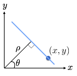
Polar representation for detecting lines using Hough Transform
When using Hough transform to detect lines, it is often preferrable to express lines passing through a point in Polar coordinates. Within this context polar representation is superior to slope-intercept (m-c) parameter space, since it the latter is unbounded.
We can express the set of lines passing through Cartesian point $(x,y)$ as follows:
$$ \rho = x \cos(\theta) + y \cos(\theta). $$
Here $\rho$ and $\theta$ describe a line in polar coordinates. $\rho$ is the perpendicular distance from the origin, and $\theta$ is angle with with horizontal.
data, extents = toy_data1()
plt.figure(figsize=(7,7))
plt.title('Data')
plt.xlabel('x')
plt.ylabel('y')
plt.scatter(data[:,0], data[:,1], c='red')
plt.xlim(extents[:2])
plt.ylim(extents[-2:]);
Setting up $\theta$ and $\rho$ parameter space
theta_min, theta_max, theta_num = 0, 2*np.pi, 1000
rho_min, rho_max, rho_num = 0.0, np.sqrt(12*12 + 12*12), 1000

print(f'theta = ({theta_min},{theta_max})')
print(f'rho = ({rho_min},{rho_max})')

theta = np.linspace(theta_min, theta_max, theta_num)
rho = np.linspace(rho_min, rho_max, rho_num)

tt, rr = np.meshgrid(theta, rho, indexing='ij')
tt = tt.flatten()
rr = rr.flatten()
theta = (0,6.283185307179586)
rho = (0.0,16.97056274847714)
dtheta = theta[1] - theta[0]
drho = rho[1] - rho[0]
print(f'dtheta = {dtheta}')
print(f'drho = {drho}')
dtheta = 0.006289474781961547
drho = 0.016987550298775914
def raster_hough_polar(data, counts, rr, tt, drho):
    theta_num, rho_num = counts.shape
    n = data.shape[0]
    for i in range(n):
        x = data[i,0]
        y = data[i,1]

        estimated_rho = x * np.cos(tt) + y * np.sin(tt)
        diffs = np.abs(estimated_rho - rr)
        votes = diffs <= drho
        votes = votes.astype('int').reshape(theta_num, rho_num)
        counts = counts + votes
    return counts
Collecting votes in Hough space
counts = np.zeros((theta_num, rho_num))
counts = raster_hough_polar(data, counts, rr, tt, drho)
plt.figure(figsize=(12,12))
plt.title('Hough space')
plt.imshow(counts.T, origin='lower')
plt.imshow(counts.T, origin='lower')
plt.xlabel(f'$\\Theta$ [{theta_min},{theta_max*180/np.pi}]')
plt.ylabel(f'$\\rho$ [{rho_min:5.3},{rho_max:5.3}]');

Estimating $\theta$ and $\rho$
k = 4
estimated_theta, estimated_rho = find_top_k_cells(k, counts, theta, rho)
plt.figure(figsize=(12,12))
plt.title('Hough space')
plt.xlim(theta_min, theta_max)
plt.ylim(rho_min, rho_max)
plt.scatter(estimated_theta, estimated_rho, c='red')
plt.imshow(counts.T, origin='lower')
plt.imshow(counts.T, origin='lower', extent=[theta_min, theta_max, rho_min, rho_max])
plt.xlabel(f'$\\Theta$ [{theta_min},{theta_max*180/np.pi}]')
plt.ylabel(f'$\\rho$ [{rho_min:5.3},{rho_max:5.3}]');

print(f'estimated (theta, rho) =\n{np.vstack([estimated_theta, estimated_rho]).T}')
estimated (theta, rho) =
[[2.35855304 2.10645624]
 [2.35226357 2.15741889]
 [2.35226357 2.14043134]
 [5.82405365 2.27633174]]
plt.figure(figsize=(7,7))
plt.title('Data')
plt.xlabel('x')
plt.ylabel('y')
plt.scatter(data[:,0], data[:,1], c='red')
plt.xlim(extents[:2])
plt.ylim(extents[-2:]);
for i in range(k):
    coord = np.array([
        estimated_theta[i],
        estimated_rho[i]
    ])
    draw_line_polar(coord, plt.gca())

Noisy data
data, extents = toy_data2()
plt.figure(figsize=(15,15))
plt.subplot(221)
plt.xlabel('x')
plt.ylabel('y')
plt.title('Noisy data')
plt.scatter(data[:,0], data[:,1], c='blue', alpha=0.5)
plt.xlim(extents[:2])
plt.ylim(extents[-2:]);
Collecting votes in Hough space
theta_min, theta_max, theta_num = 0, 2*np.pi, 1000
#rho_min, rho_max, rho_num = 0.0, np.sqrt(30*30 + 30*30), 1000
rho_min, rho_max, rho_num = 0.0, 25.0, 1000

print(f'theta = ({theta_min},{theta_max})')
print(f'rho = ({rho_min},{rho_max})')

theta = np.linspace(theta_min, theta_max, theta_num)
rho = np.linspace(rho_min, rho_max, rho_num)

tt, rr = np.meshgrid(theta, rho, indexing='ij')
tt = tt.flatten()
rr = rr.flatten()
theta = (0,6.283185307179586)
rho = (0.0,25.0)
dtheta = theta[1] - theta[0]
drho = rho[1] - rho[0]
print(f'dtheta = {dtheta}')
print(f'drho = {drho}')
dtheta = 0.006289474781961547
drho = 0.025025025025025027
counts = np.zeros((theta_num, rho_num))
counts = raster_hough_polar(data, counts, rr, tt, drho)
plt.figure(figsize=(12,12))
plt.title('Hough space')
plt.imshow(counts.T, origin='lower')
plt.imshow(counts.T, origin='lower')
plt.xlabel(f'$\\Theta$ [{theta_min},{theta_max*180/np.pi}]')
plt.ylabel(f'$\\rho$ [{rho_min:5.3},{rho_max:5.3}]');

nbins_theta = 32
nbins_rho = 32

edges_theta = np.linspace(theta_min, theta_max, nbins_theta)
edges_rho = np.linspace(rho_min, rho_max, nbins_rho)

width_edges_theta = edges_theta[1] - edges_theta[0]
width_edges_rho = edges_rho[1] - edges_rho[0]
plt.figure(figsize=(10,10))
ax = plt.subplot(111, title='Visualizing 2D grid')
ax.set_xlim(theta_min, theta_max)
ax.set_xticks(edges_theta, minor=True)
ax.xaxis.grid(True, which='minor')
ax.set_ylim(rho_min, rho_max)
ax.set_yticks(edges_rho, minor=True)
ax.yaxis.grid(True, which='minor')
plt.imshow(counts.T, origin='lower', extent=[theta_min, theta_max, rho_min, rho_max])
plt.xlabel('m')
plt.ylabel('c');

H, _, _ = np.histogram2d(tt, rr, weights=counts.ravel(), bins=(edges_theta, edges_rho))
k = 3

H_ = H.ravel()
cell_loc_ = H_.argsort()[::-1][:k]
cell_loc_i, cell_loc_j = np.unravel_index(cell_loc_, H.shape)

estimated_theta = edges_theta[cell_loc_i] + (width_edges_theta*0.5)
estimated_rho = edges_rho[cell_loc_j] + (width_edges_rho*0.5)
fig = plt.figure(figsize=(10, 10))
ax = fig.add_subplot(111, title='Visualizing histogram as an image')
plt.imshow(H.T, interpolation='nearest', origin='lower', extent=[edges_theta[0], edges_theta[-1], edges_rho[0], edges_rho[-1]], cmap='Spectral')
plt.colorbar();

plt.figure(figsize=(10,10))
ax = plt.subplot(111, aspect=True)
plt.xlabel('x')
plt.ylabel('y')
plt.title('Picking the best lines')
plt.xlim(extents[:2])
plt.ylim(extents[-2:])
for i in range(k):
    coord = np.array([estimated_theta[i], estimated_rho[i]])
    draw_line_polar(coord, ax, alpha=0.9, c='red')
plt.scatter(data[:,0], data[:,1], c='blue', alpha=0.5);

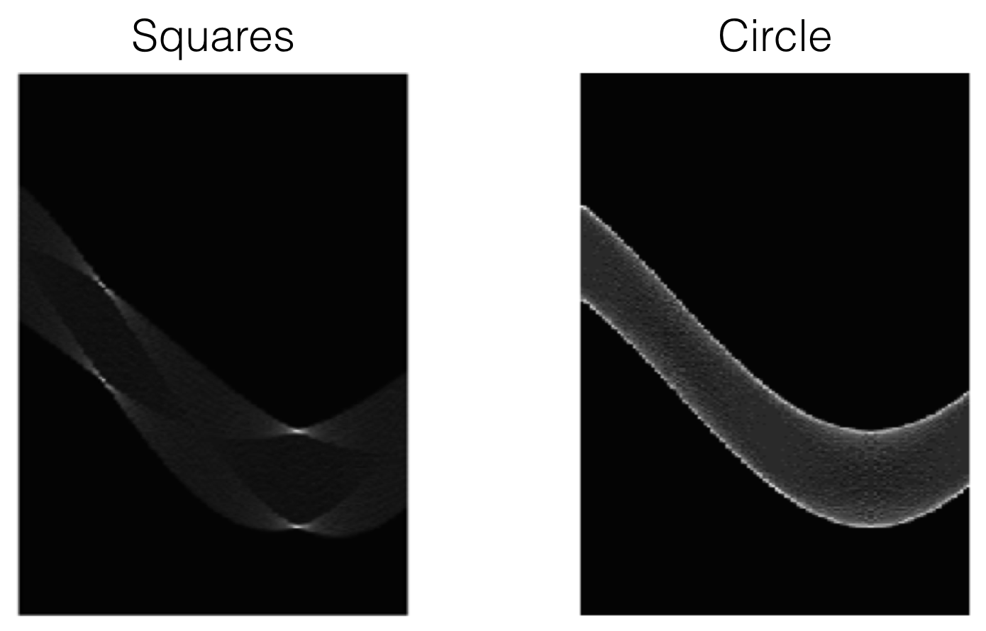
Discussion
Examples
Dealing with noisy data
- Choose a good grid size (or discretization)
- Too small: miss lines because only points that are exactly collinear will vote for a single line
- Too large: many different lines will appear in the same bucket
- Increment neighbouring bins (smoothing accumulator arrays)
- Avoid irrelevant features.
- Use pixels on strong edges (e.g., selected via gradient magnitude)
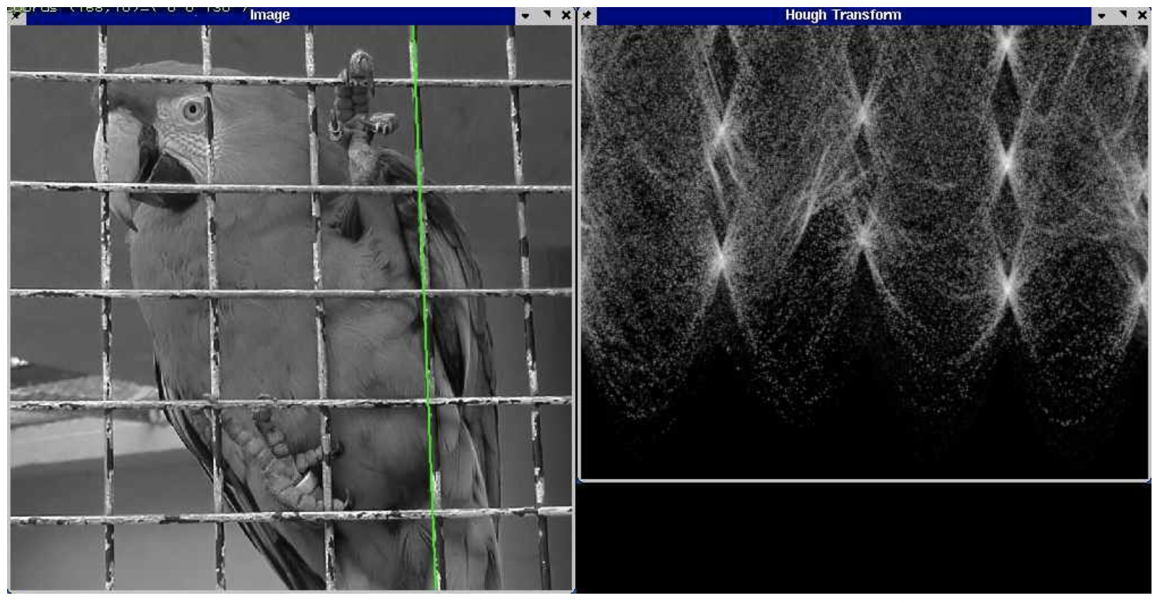
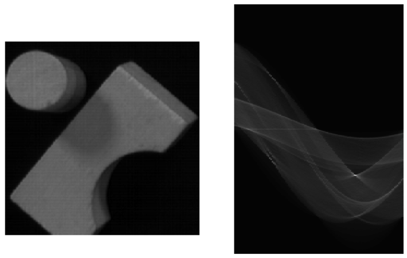
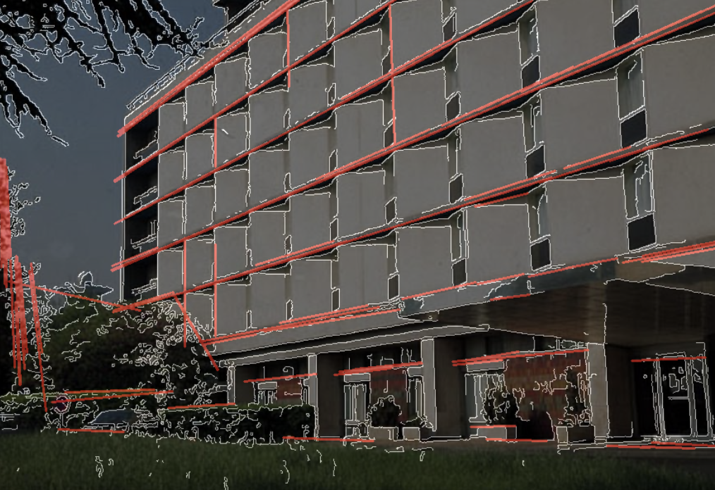
OpenCV Hough transform example
Generalized hough transform
Readings
- D. Ballard and C. Brown Computer Vision, Prentice-Hall, 1982, Chap. 4.
- R. Boyle and R. Thomas Computer Vision:A First Course, Blackwell Scientific Publications, 1988, Chap. 5.
- A. Jain Fundamentals of Digital Image Processing, Prentice-Hall, 1989, Chap. 9.
- D. Vernon Machine Vision, Prentice-Hall, 1991, Chap. 6.