Image Pyramids

Faisal Qureshi
Professor
Faculty of Science
Ontario Tech University
Oshawa ON Canada
http://vclab.science.ontariotechu.ca

Copyright information

© Faisal Qureshi

License

This work is licensed under a Creative Commons Attribution-NonCommercial 4.0 International License.

Lesson Plan

• Gaussian image pyramids
• Laplacian image pyramids
• Laplacian blending

Uses

Often used to achieve scale-invariant processing in the following contexts:

• template matching;
• image registration;
• image enhancement;
• interest point detection; and
• object detection.

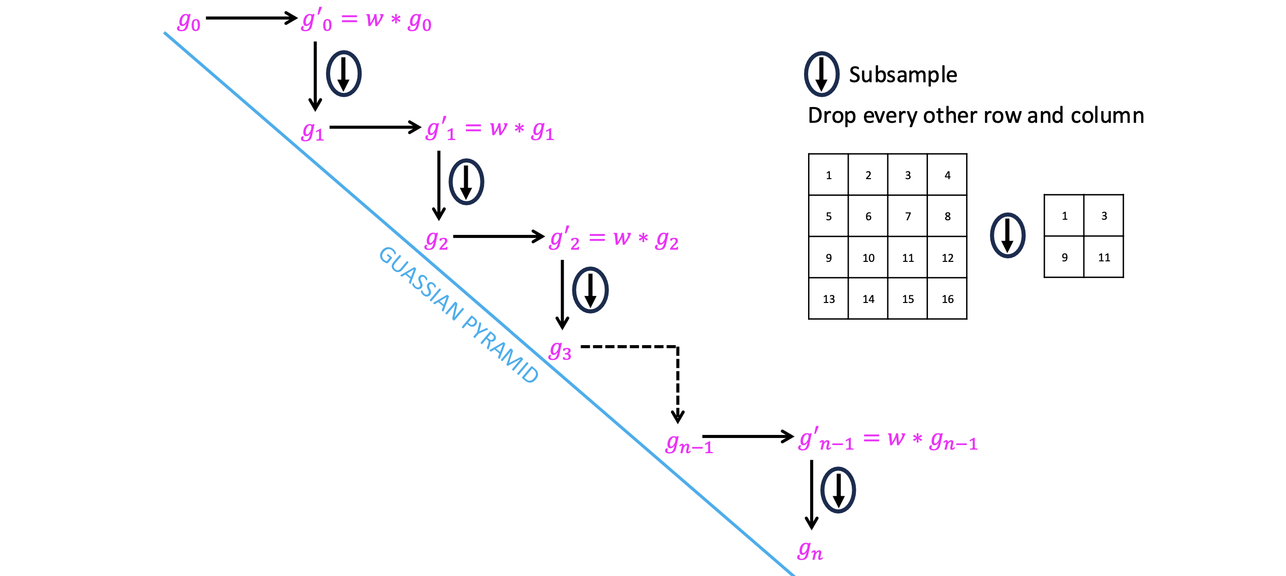
Gaussian Image Pyramid

The basic idea for constructing Gaussian image pyramid is as follows:

Let $g_0 = I$ and $i = 0$

1. Blur $g_i$ with a Gaussian kernel $w$ to create $g'_i$
2. Reduce $g'_i$ dimensions by half by discarding every other row and and every other column to construct $g_{i+1}$
3. Set $i = i+1$ and repeat this process until desired numbers levels are achieved or the image is reduced to size $1 \times 1$

Courtesy D. Forsyth

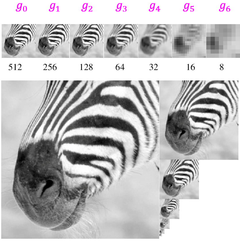
Starting with $g_0 = I$ the following figure depicts the construction of a Gaussian Pyramid.

import numpy as np
import math
import cv2 as cv
import matplotlib.pyplot as plt

Exercise 04-01

• Load image 'data/apple.jpg'
• Blur each channel with a 5-by-5 Gaussian kernel
• Construct the next level of Gaussian pyramid by discarding every other row or column

Solution:

# %load solutions/image-pyramids/solution_01.py
#I = cv.imread('data/apple.jpg')
I = cv.imread('data/van-gogh.jpg')
I = cv.cvtColor(I, cv.COLOR_BGR2RGB)
I = cv.resize(I, (512, 512))

print('Shape of I = {}'.format(I.shape))

I[:,:,0] = cv.GaussianBlur(I[:,:,0], (5,5), 2, 2)
I[:,:,1] = cv.GaussianBlur(I[:,:,1], (5,5), 2, 2)
I[:,:,2] = cv.GaussianBlur(I[:,:,2], (5,5), 2, 2)

I2 = I[::2,::2,:]
print('Shape of I2 = {}'.format(I2.shape))

plt.imshow(I2);

Shape of I = (512, 512, 3)
Shape of I2 = (256, 256, 3)

Implementation (Gaussian Image Pyramid)

# %load solutions/image-pyramids/gen_gaussian_pyramid.py 
def gen_gaussian_pyramid(I, levels=6):
    G = I.copy()
    gpI = [G]
    for i in range(levels):
        G = cv.pyrDown(G)
        gpI.append(G)
    return gpI

# %load solutions/image-pyramids/gen_gaussian_pyramid.py 
def gen_pyramid(I, levels=6):
    G = I.copy()
    pI = [G]
    for i in range(levels):
        G = G[::2,::2,:]
        pI.append(G)
    return pI

foo = gen_gaussian_pyramid(I, levels=9)
boo = gen_pyramid(I, levels=9)

for i in foo:
    print(i.shape)

for i in boo:
    print(i.shape)

(512, 512, 3)
(256, 256, 3)
(128, 128, 3)
(64, 64, 3)
(32, 32, 3)
(16, 16, 3)
(8, 8, 3)
(4, 4, 3)
(2, 2, 3)
(1, 1, 3)
(512, 512, 3)
(256, 256, 3)
(128, 128, 3)
(64, 64, 3)
(32, 32, 3)
(16, 16, 3)
(8, 8, 3)
(4, 4, 3)
(2, 2, 3)
(1, 1, 3)

def show_pyramid(p):
    n = len(p)
    for i in range(n):
        c = 4
        r = math.ceil(n / c)
        ax = plt.subplot(r,c,i+1)
        ax.imshow(p[i])

plt.figure(figsize=(20,15))
plt.title('Without Gaussian Blurring')
show_pyramid(boo)

plt.figure(figsize=(20,15))
plt.title('Gaussian Blurring')
show_pyramid(foo)

Kernel for Gaussian blurring

OpenCV pyrDown method performs steps 1 and 2 above. It uses the following kernel to blur the image (in step 1).

$$ \frac{1}{256} \left[ \begin{array}{ccccc} 1 & 4 & 6 & 4 & 1 \\ 4 & 16 & 24 & 16 & 4 \\ 6 & 24 & 36 & 24 & 6 \\ 4 & 16 & 24 & 16 & 4 \\ 1 & 4 & 6 & 4 & 1 \end{array} \right] $$

A = cv.imread('data/apple.jpg')
B = cv.imread('data/orange.jpg')
A = cv.cvtColor(A, cv.COLOR_BGR2RGB)
B = cv.cvtColor(B, cv.COLOR_BGR2RGB)

gpA = gen_gaussian_pyramid(A)
gpB = gen_gaussian_pyramid(B)

gp = gpB
num_levels = len(gp)
for i in range(num_levels):
    rows = gp[i].shape[0]
    cols = gp[i].shape[1]
    print('level={}: size={}x{}'.format(i, rows, cols))

level=0: size=512x512
level=1: size=256x256
level=2: size=128x128
level=3: size=64x64
level=4: size=32x32
level=5: size=16x16
level=6: size=8x8

gp = gpA
level = 3
plt.figure(figsize=(10,10))
plt.title('Level {}'.format(level))
plt.imshow(gp[level])

<matplotlib.image.AxesImage at 0x1121e5810>

Laplacian operator

We define Laplacian operator as follows:

$$ \nabla^2 f = \frac{\partial^2 f}{\partial x^2} + \frac{\partial^2 f}{\partial y^2} $$

Approximation

In addition we can approximate the Laplacian of a Gaussian as follows:

Source: Lazebnik

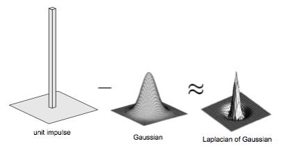
We use this property when constructing Laplacian image pyramids above.

Laplacian of a Gaussian

Approach 1: via computing derivatives

# 1D kernel for computing derivatives
Hx = np.array([1,-1], dtype='float32')

s = 4
ticks = np.linspace(-s,s,2*s+1)

gxx = np.linspace(-40,40,801)
mu = 0
sigma = 5
g = np.exp(- (gxx-mu)**2 / (2*(sigma**2)) ) / ( 2 * np.pi * sigma)

plt.figure(figsize=(20,5))
plt.plot(gxx, g, 'k', linewidth=5)
plt.xlim([-s*sigma, s*sigma])
plt.yticks([])
plt.title(r'Gaussian.  ($\mu=0, \sigma=5$)');

dg = np.convolve(g, Hx, 'same')

plt.figure(figsize=(20,5))
plt.plot(gxx, dg, 'k', linewidth=5)
plt.xlim([-s*sigma, s*sigma])
plt.yticks([])
plt.title(r'Gaussian 1st derivative.  ($\mu=0, \sigma=5$)');

ddg = np.convolve(dg, Hx, 'same')

plt.figure(figsize=(20,5))
plt.plot(gxx, ddg, 'k', linewidth=5)
plt.xlim([-s*sigma, s*sigma])
plt.yticks([])
plt.title(r'Gaussian Laplacian computed via 2nd derivative.  ($\mu=0, \sigma=5$)');

Approach 2: approximating Laplacian of a Gaussian

G_kernel = np.array([1., 4., 6., 4., 1.]) / 16.
g_smoothed = np.convolve(G_kernel, g, 'same')

s = 4
ticks = np.linspace(-s,s,2*s+1)

gxx = np.linspace(-40,40,801)
mu = 0
sigma = 5
g = np.exp(- (gxx-mu)**2 / (2*(sigma**2)) ) / ( 2 * np.pi * sigma)

G_kernel = np.array([1., 4., 6., 4., 1.]) / 16.
g_smoothed = np.convolve(G_kernel, g, 'same')

plt.figure(figsize=(20,5))
plt.plot(gxx, g_smoothed-g, 'k', linewidth=5, label='approximation')
plt.plot(gxx, ddg, 'k', linewidth=1, label='2nd derivative')
plt.xlim([-s*sigma, s*sigma])
plt.yticks([])
plt.legend()
plt.title(r'Gaussian Laplacian approximation.  ($\mu=0, \sigma=5$)');

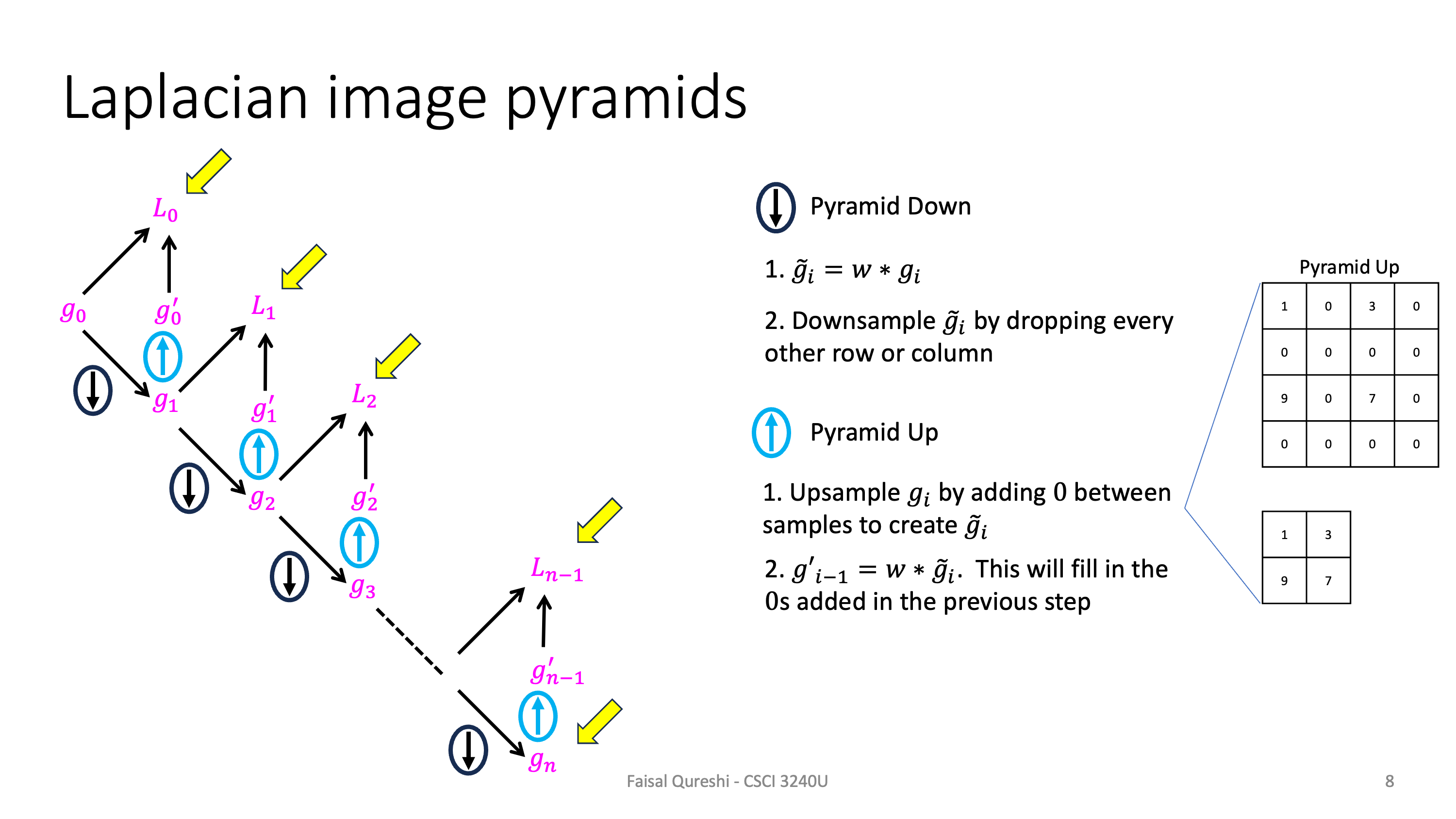
Laplacian Image Pyramid

Proposed by Burt and Adelson is a bandpass image decomposition derived from the Gaussian pyramid. Each level encodes information at a particular spatial frequency. The basic steps for constructing Laplacian pyramids are:

Construction (for image $I$)

Let $g_0 = I$ and set $i = 0$

1. Convolve $g_i$ with Gaussan kernel (low-pass filter $w$) and down-sample by half to construct $g_{i+1}$. Downsample by discarding every other row and column.
2. Upsample $g_{i+1}$ by inserting $0$s between each row and column and interpolating the missing values by convolving it with $w$ and create $g'_i$
3. Compute $L_i = g_i - g'_i$
4. Set $i = i+1$ and repeat till the desired levels are reached.

Courtesy D. Forsyth

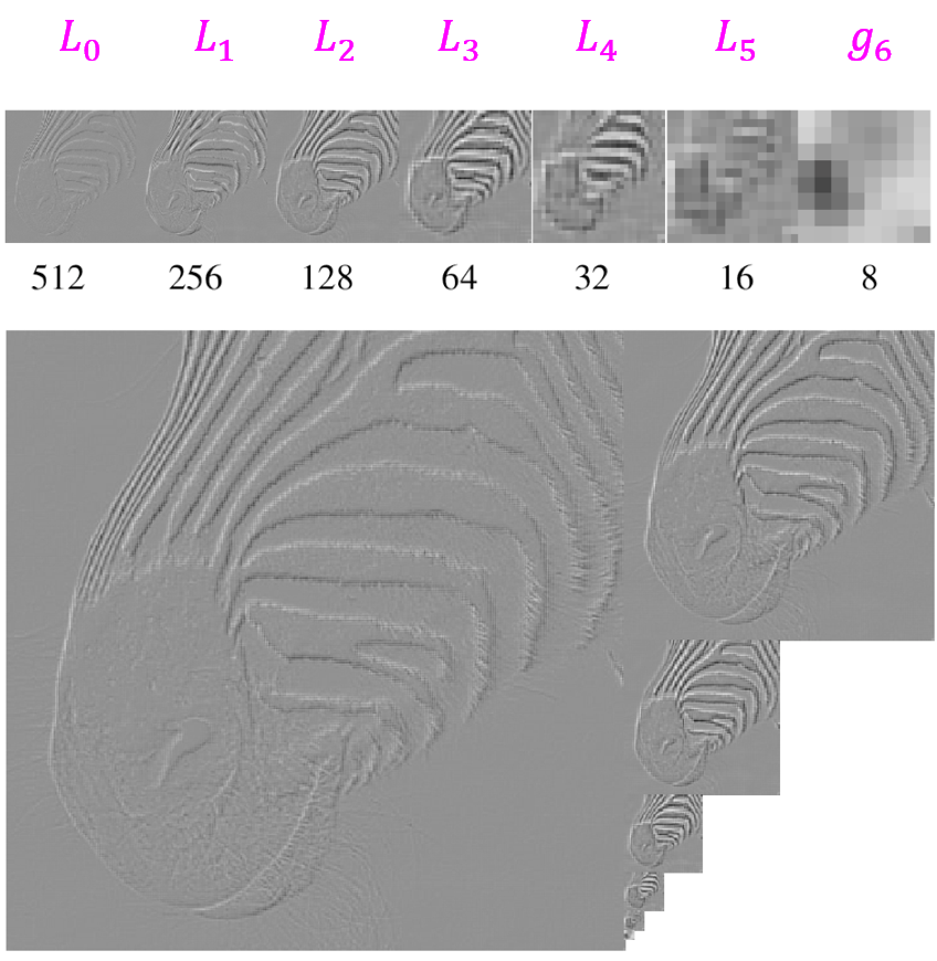
Starting with image $I$, the following figure illustrates the construction of Laplacian pyramid.

Reconstructing the original image

It is possible to reconstruct the original image $I$ from its Laplacian image pyramid consisting of $n$ levels: $\{L_0, L_1, \cdots, L_{n-1}, g_n \}$.

Set $i=n$

1. Upsample $g_i$ by inserting zeros between sample values and interpolate the missing values by convolving it with a filter $w$ to get $g'_{i-1}$.
2. Set $g_{i-1} = L_{i-1} + g'_{i-1}$.
3. Set $i = i-1$ and repeat till $i = 0$
4. Set $I = g_0$

Uses

Laplacian image pyramids are often used for compression. Instead of encoding $g_0$, we encode $L_i$, which are decorrelated and can be represented using far fewer bits.

Implementation (Laplacian Image Pyramid)

# %load solutions/image-pyramids/gen_laplacian_pyramid.py
def gen_laplacian_pyramid(gpI):
    """gpI is a Gaussian pyramid generated using gen_gaussian_pyramid method found in py file of the same name."""
    num_levels = len(gpI)-1
    lpI = [gpI[num_levels]]
    for i in range(num_levels,0,-1):
        GE = cv.pyrUp(gpA[i])
        L = cv.subtract(gpA[i-1],GE)
        lpI.append(L)
    return lpI

lpA = gen_laplacian_pyramid(gpA)
lpB = gen_laplacian_pyramid(gpB)

lp = lpA
num_levels = len(lp)
for i in range(num_levels):
    rows = lp[i].shape[0]
    cols = lp[i].shape[1]
    print('level={}: size={}x{}'.format(i, cols, rows))

level=0: size=8x8
level=1: size=16x16
level=2: size=32x32
level=3: size=64x64
level=4: size=128x128
level=5: size=256x256
level=6: size=512x512

plt.figure(figsize=(20,10))
plt.title('Laplacian Pyramid')
show_pyramid(lpA)

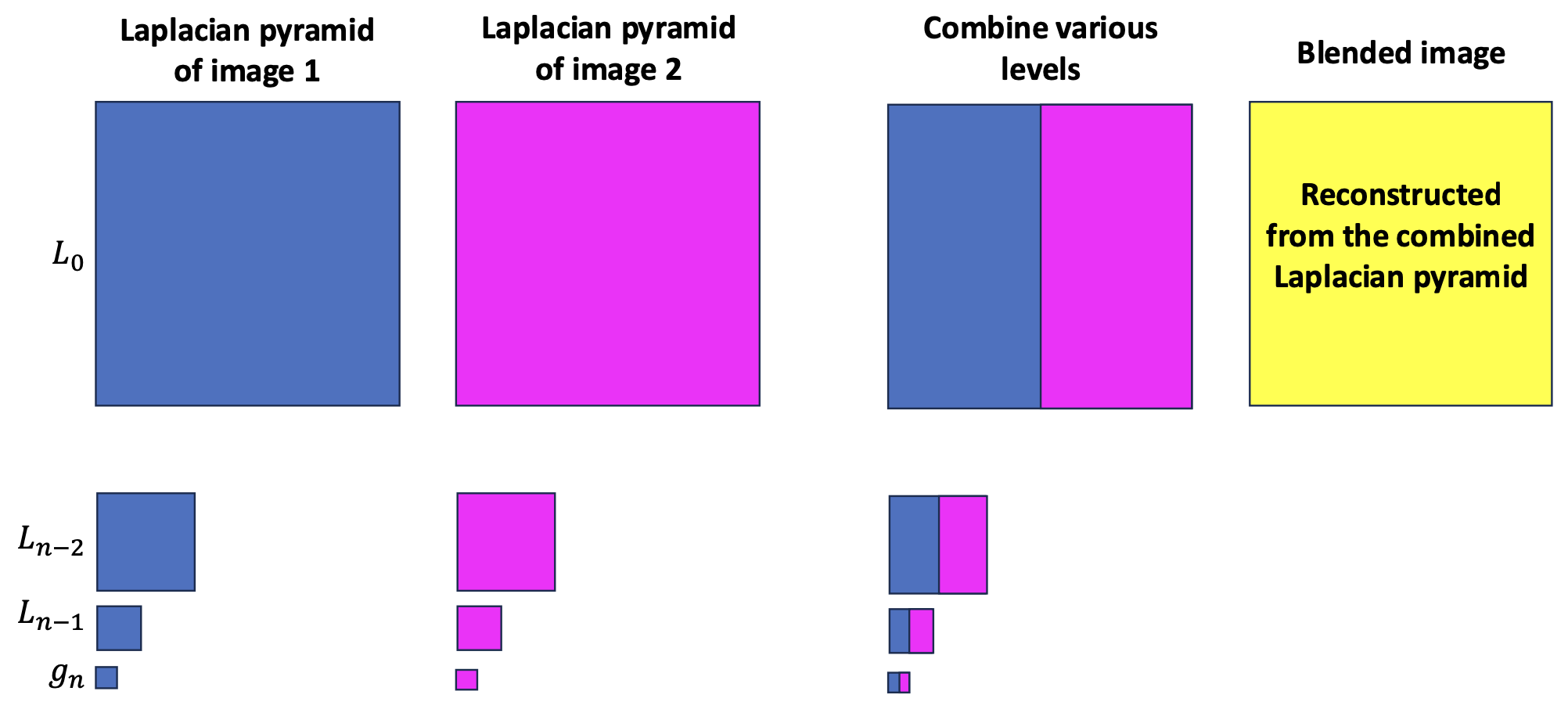
Laplacian Blending

Constructing Laplacian Pyramid of First Image

plt.figure(figsize=(20,10))
plt.title('Laplacian Pyramid of Apple')
show_pyramid(lpA)

Constructing Laplacian Pyramid of Second Image

plt.figure(figsize=(20,10))
plt.title('Laplacian Pyramid of Orange')
show_pyramid(lpB)

Blending

# %load solutions/image-pyramids/laplacian_blending.py
LS = []
for la, lb in zip(lpA, lpB):
    rows, cols, dpt = la.shape
    ls = np.hstack((la[:,0:cols//2,:], lb[:,cols//2:,:]))
    LS.append(ls)

plt.figure(figsize=(20,10))
plt.title('Laplacian Pyramid Blended')
show_pyramid(LS)

Reconstruction

# %load solutions/image-pyramids/reconstruct_from_laplacian.py
ls_ = LS[0]
for i in range(1,6):
    ls_ = cv.pyrUp(ls_)
    ls_ = cv.add(ls_, LS[i])

plt.figure(figsize=(10,10))
plt.imshow(ls_)

<matplotlib.image.AxesImage at 0x113aabd90>

Blending without Laplacian Pyramids

real = np.hstack((A[:,:cols//2],B[:,cols//2:]))

plt.figure(figsize=(10,10))
plt.imshow(real);

Conclusions and Summary

• Gaussian pyramid
  • Coarse-to-fine search
  • Multi-scale image analysis (hold this thought)

• Laplacian pyramid
  • More compact image representation
  • Can be used for image compositing (computation photography)

• Downsampling
  • Nyquist limit: The Nyquist limit gives us a theoretical limit to what rate we have to sample a signal that contains data at a certain maximum frequency. Once we sample below that limit, not only can we not accurately sample the signal, but the data we get out has corrupting artifacts. These artifacts are "aliases".
  • Need to sufficiently low-pass before downsampling

Various image representations

• Pixels: great for spatial processing, poor access to frequency
• Fourier transform: great for frequency analysis, poor spatial info (soon)
• Pyramids: trade-off between spatial and frequency information

Playground

I = cv.imread('data/flowers-minhas.jpg', 0)
print(I.shape)

(683, 1024)

plt.figure(figsize=(5,5))
plt.imshow(I, cmap='grey')

<matplotlib.image.AxesImage at 0x113b939d0>

# def gen_gaussian_pyramid(I, levels=6):
#     G = I.copy()
#     gpI = [G]
#     for i in range(levels):
#         G = cv.pyrDown(G)
#         gpI.append(G)
#     return gpI

G0 = I.copy()
G1 = cv.pyrDown(G0)
G2 = cv.pyrDown(G1)

plt.figure(figsize=(15,5))
plt.subplot(131)
plt.imshow(G0, cmap='gray')
plt.subplot(132)
plt.imshow(G1, cmap='gray')
plt.subplot(133)
plt.imshow(G2, cmap='gray')

<matplotlib.image.AxesImage at 0x113b46990>

print('G0', G0.shape)
print('G1', G1.shape)
print('G2', G2.shape)

G0_prime = cv.pyrUp(G1)
h = np.min([G0.shape[0],G0_prime.shape[0]])
w = np.min([G0.shape[1],G0_prime.shape[1]])
print(h,w)
E = np.empty(G0.shape)
E[0:h,0:w] = G0_prime[0:h,0:w]
print(E.shape)
L0 = G0 - E

G1_prime = cv.pyrUp(G2)
h = np.min([G1.shape[0],G1_prime.shape[0]])
w = np.min([G1.shape[1],G1_prime.shape[1]])
print(h,w)
E = np.empty(G1.shape)
E[0:h,0:w] = G1_prime[0:h,0:w]
print(E.shape)
L1 = G1 - E

G2 = G2

plt.figure(figsize=(15,5))
plt.subplot(131)
plt.imshow(L0, cmap='gray')
plt.subplot(132)
plt.imshow(L1, cmap='gray')
plt.subplot(133)
plt.imshow(G2, cmap='gray')

G0 (683, 1024)
G1 (342, 512)
G2 (171, 256)
683 1024
(683, 1024)
342 512
(342, 512)

<matplotlib.image.AxesImage at 0x113e716d0>

G1_prime = cv.pyrUp(G2)
h = np.min([L1.shape[0],G1_prime.shape[0]])
w = np.min([L1.shape[1],G1_prime.shape[1]])
print(h,w)
E = np.empty(L1.shape)
E[0:h,0:w] = G1_prime[0:h,0:w]
print(E.shape)
G1 = L1 + E

G0_prime = cv.pyrUp(G1)
h = np.min([L0.shape[0],G0_prime.shape[0]])
w = np.min([L0.shape[1],G0_prime.shape[1]])
print(h,w)
E = np.empty(L0.shape)
E[0:h,0:w] = G0_prime[0:h,0:w]
print(E.shape)
G0 = L0 + E

plt.figure(figsize=(5,5))
plt.imshow(G0, cmap='grey')

342 512
(342, 512)
683 1024
(683, 1024)

<matplotlib.image.AxesImage at 0x113f5de50>

plt.figure(figsize=(5,5))
plt.imshow(np.abs(I-G0), cmap='grey')
plt.colorbar()

<matplotlib.colorbar.Colorbar at 0x110a8fe00>