Linear Filtering

Faisal Qureshi
Professor
Faculty of Science
Ontario Tech University
Oshawa ON Canada
http://vclab.science.ontariotechu.ca

Copyright information

© Faisal Qureshi

License

This work is licensed under a Creative Commons Attribution-NonCommercial 4.0 International License.

Lesson Plan

• Linear Filtering in 1D
• Cross-correlation
• Convolution
• Gaussian filter
• Gaussian blurring
• Separability
• Relationship to Fourier transform
• Integral images

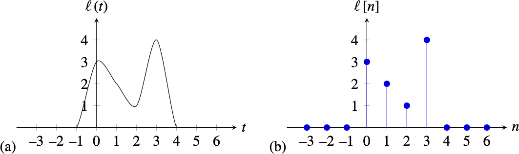
Continuous and Discrete Signals

Most of the signals that exist in nature are infinite continuous signals, when we introduce them into a computer they are sampled and transformed into a finite sequence of numbers, also called a discrete signal.

Credit: Foundations of Computer Vision

Average (DC) value of a signal

For discrete signals $x$ of length $N$ $$ \mu = \frac{1}{N} \sum_{n=0}^{N-1} x[n] $$

For continuous signals $$ \mu = \lim_{T \rightarrow \infty} \frac{1}{2T+1} \sum_{t=-T}^{T} x(t) $$

Comparing two signals

We can use Euclidean distance

$$ D^2 = \frac{1}{N} \sum_{n=0}^{N-1} | x_1[n] - x_2[n] |^2 $$

This is not the only way we can compare two signals.

Signal Power

For discrete signals $x$ of length $N$ $$ P_x = \frac{1}{N} \sum_{n=0}^{N-1} |x[n]|^2 $$

For continuous signals $$ P_x = \lim_{T \rightarrow \infty} \frac{1}{2T+1} \sum_{t=-T}^{T} |x(t)|^2 $$

Linear Systems

Consider a function (system) $f$ that takes in $x$ and returns $y$

Credit: Foundations of Computer Vision

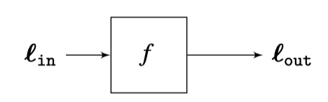
A system is any mathematical or physical process that transforms a signal. For example, an audio amplifier, biological vision system, image blur filters, a fully-connected layer in a neural network, etc.

Linear systems is a small subset of all possible systems, it satisfies the Principle of Superposition:

• Addititivity: $f(x_1 + x_2) = f(x_1) + f(x_2)$
• Homogeneity (Scaling): $f(ax) = af(x)$ for any scalar $a$

In a linear system the rules can change over time. Consider an audio amplifier. At each instant, its response is linear however a user can use the volume knob to change the gain. So, the system response is not constant.

Linear Translation Invariant Systems (LTIs)

A system is a linear translation invariant system if it is (1) linear and (2) when we translate the input signal by $n_0$, the output is also translated by $n_0$

$$ y[n-n_0] = f(x[n-n_0]) $$

This property is referred to as equivariant with respect to translation. Or more generally, for LTIs, the system behavior is constant. It reacts to the signal the same way regardless of when the signal arrives.

Convolution

The Unit Impulse ($\delta$)

Unit Impulse (Dirac Delta Function) is defined as

$$ \delta(t) = 0\;\;\text{for}\;\;t \neq 0 $$ where $\int_{-\infty}^{\infty} \delta(t) dt = 1$ (Unit Area).

$\delta$ is infinitely high with zero width. Thinking in terms of Fourier domain, $\delta$ contains all frequencies.

Physical Analogy: An instantaneous hit, like a hammer strike or a handclap.

If we multiply any signal $x(t)$ by an impulse $\delta(t-\tau)$, it grabs the value of that signal at each time $\tau$.

Impulse Response: $h(t)$

The specific output produced when a unit impulse is fed into a system.

It is the "DNA" of an LTI system. For example, it is possible to characterize the acoustic properties of a room by simply clapping once (the unit impulse) and recording the resulting sound (the impulse response).

Representing a system as a sum of impulses

We can represent a signal as a sum of impulses $$ x(t) = \int_{-\infty}^{\infty} x(\tau) \delta(t - \tau) d \tau. $$ Here $x(\tau)$ is the amplitude of impulse at time $\tau$.

For discrete signals $$ x[n] = \sum_{k=-\infty}^{\infty} x[k] \delta[n - k]. $$ where $\delta[n-k]$ is the Kronecker Delta which is non-zero everywhere except at $n=k$.

Linear systems

If we represent our system as an operator $H$ then $$ H \left[ x(t) \right] = H \left[ \int_{-\infty}^{\infty} x(\tau) \delta(t - \tau) d \tau \right]. $$ Since $H$ is linear, we can move it inside the integral (which is simply a sum of scaled values) $$ H \left[ x(t) \right] = \int_{-\infty}^{\infty} x(\tau) H \left[ \delta(t - \tau) \right] d \tau . $$ $H \left[ \delta(t - \tau) \right]$ denotes the impulse of the system that happens at time $\tau$. It is sometimes referred to as time-varying impulse response $h(t, \tau)$. Specifically $$ H \left[ x(t) \right] = \int_{-\infty}^{\infty} x(\tau) h(t, \tau) d \tau . $$ In a linear system, the system's response to an impulse can look different at different times. An echo in a room may sound different at 2 pm and at 8 pm.

LTI (Continuous Signals)

In linear translation invariant system, however, the response to a shifted impulse $\delta(t - \tau)$ is simply shifted version of the response to impulse $\delta(t)$. If we define $h(t) = H[\delta(t)]$ then $H[\delta(t-\tau)]=h(t-\tau)$.

So for LTI system we have $$ H \left[ x(t) \right] = \int_{-\infty}^{\infty} x(\tau) h(t-\tau) d \tau . $$ This is the convolution integral often written as $$ y(t) = x(t) \ast h(t) $$ where $y(t) = H \left[ x(t) \right]$, i.e., the value of the output signal at time $t$.

This has important consequences: (1) linearity allows us to break the signal into pieces and sum the results and (2) translation invariance ensures that every piece reacts the same way, regardless of when it arrives. Without translation invariance, we would need a different impulse response $h(t, \tau)$ for every single point in time. With it, we only need on function $h(t)$ to know everything about the system.

Convolution is Commutative

Goal: Prove that $x(t) * h(t) = h(t) * x(t)$.

Step 1: Definition Start with the standard definition of the convolution integral: $$x(t) * h(t) = \int_{-\infty}^{\infty} x(\tau) h(t - \tau) \, d\tau$$

Step 2: Change of Variables We introduce a new variable $u$ to replace the time-shifted argument inside $h$. Let: $$u = t - \tau$$

This implies: $$\tau = t - u$$ $$d\tau = -du$$

Step 3: Change of Limits We must transform the limits of integration from $\tau$ to $u$:

• As $\tau \to -\infty$, $u \to \infty$
• As $\tau \to \infty$, $u \to -\infty$

Step 4: Substitution Substitute $\tau$, $d\tau$, and the limits into the integral: $$x(t) * h(t) = \int_{\infty}^{-\infty} x(t - u) h(u) \, (-du)$$

Step 5: Simplify Use the negative sign on the differential $(-du)$ to flip the limits of integration back to the standard order ($-\infty$ to $\infty$): $$= \int_{-\infty}^{\infty} x(t - u) h(u) \, du$$

Rearrange the terms inside the integral (multiplication is commutative): $$= \int_{-\infty}^{\infty} h(u) x(t - u) \, du$$

Conclusion This final expression matches the definition of $h(t) * x(t)$. $$x(t) * h(t) = h(t) * x(t) \quad \text{Q.E.D.}$$

LTI (Discrete Signals)

We can re-write the convolution integral as $$ y[n] = x[n] \ast h[n] = \sum_{k=-\infty}^{\infty} x[k] h[n-k]. $$ This is sometimes referred to as the convolution sum formula.

Convolution is Commutative

Goal: Prove that $x[n] * h[n] = h[n] * x[n]$.

Step 1: Definition Start with the convolution sum formula: $$x[n] * h[n] = \sum_{k=-\infty}^{\infty} x[k] h[n - k]$$

Step 2: Change of Index Let a new index $m$ replace the argument inside $h$. Let: $$m = n - k$$

This implies: $$k = n - m$$

Step 3: Change of Summation Limits Since the sum covers all integers from $-\infty$ to $\infty$, the range remains the same, though the direction technically flips:

• As $k \to -\infty$, $m \to \infty$
• As $k \to \infty$, $m \to -\infty$

Step 4: Substitution Substitute $k$ into the sum: $$x[n] * h[n] = \sum_{m=\infty}^{-\infty} x[n - m] h[m]$$

Step 5: Simplify Because summation is commutative and covers the entire integer line, the order of limits (positive to negative vs negative to positive) does not change the result. We re-order standardly: $$= \sum_{m=-\infty}^{\infty} x[n - m] h[m]$$

Rearrange terms: $$= \sum_{m=-\infty}^{\infty} h[m] x[n - m]$$

Conclusion This matches the definition of $h[n] * x[n]$. $$x[n] * h[n] = h[n] * x[n] \quad \text{Q.E.D.}$$

Calculating $y[n]$

Cummutative property: The order does not matter; therefore, $x[n] \ast h[n] = h[n] \ast x[n]$. Therefore, $$ y[n] = x[n] \ast h[n] = \sum_{k=-\infty}^{\infty} x[n-k] h[k]. $$

Say, $h$ is defined over $-w,\cdots,0,\cdots,w$, we can re-write the above expression as $$ y[n] = x[n] \ast h[n] = \sum_{k=-w}^{w} x[n-k] h[k]. $$ This expression gives the value of output at $n$.

Why do we care?

Linear translation invariant systems are very important to us. These are motivated by the observation that we often want to process an image in a spatially invariant manner. Under translation equivariance, linear systems are equivalent to convolution with a suitable kernel. A fair bit of image processing algorithms require us to convolve an image with a suitable kernel. E.g., we can use convolution to sharpen an image, blur an image, find edges in an image, etc.

Also, don't forget that the deep learnig success story started with nothing other then ... convolutional neural networks.

Playing with an image

import numpy as np
import scipy as sp
from scipy import signal
import cv2 as cv
import matplotlib.pyplot as plt

# Load image of Van Gogh, convert from BGR to RGB image
I = cv.imread('data/van-gogh.jpg')
I = cv.cvtColor(I, cv.COLOR_BGR2RGB)

plt.figure(figsize=(7,7))
plt.imshow(I)
plt.xticks([])
plt.yticks([]);

Let's plot a single row of the red channel of image $I$, say, row 200. This is our 1D signal.

row = 200
rowI = I[row,:,0]
plt.figure()
plt.plot(rowI,'-')
plt.plot(rowI,'r.');

Using kernel to compute mean

Note here that what we have is an LTI.

signal = rowI[0:5]
kernel = np.array([1,1,1,1,1]) / 5

print(rowI[0:5])
print('A = ', np.mean(rowI[0:5]))
print('B = ', np.dot(kernel, signal))

[133 127 120 119 125]
A =  124.8
B =  124.80000000000001

Performing moving averages

Let's perform a moving average on this row. We assume window with half-width equal to $w$.

This is an example of LTI. Original data is $l_\text{in}$. The smoothed version is $l_\text{out}$.

width = 5
signal = rowI
kernel = np.ones(2*width+1)/(2*width+1) # Array to represent the window (constant-valued)
result = np.ones(len(signal)-2*width)   # Array to store computed moving averages
for i in range(len(result)):
    centre = i + width
    result[i] = np.dot(kernel, signal[centre-width:centre+width+1])

# Generate a plot of the original 1D signal and its average
plt.figure()
plt.plot(signal,'r.', alpha=0.3)
plt.plot(signal,'-', alpha=0.3)
plt.plot(np.arange(width, len(signal)-width),result,'k-');

Linear Filtering in 1D

• Signal: $\mathbf{f}$
• Kernel (also sometimes called a filter or a mask): $\mathbf{h}$
• Half-width of the kernel: $w$ (i.e., kernel width is $2 w + 1$)

Cross-Correlation

$$ CC(i) = \sum_{k \in [-w,w]} \mathbf{f}(i + k) \mathbf{h}(k) $$

Convolution

$$ (\mathbf{f} \ast \mathbf{k} )_i = \sum_{k \in [-w,w]} \mathbf{f}(i - k) \mathbf{h}(k) $$

Flipping kernel

Convolution and cross-correlation give the same results for symmetric kernels

kernel = np.array([3,1,2,1,3])
flipped_kernel = np.flip(kernel)
print('Symmetric kernel')
print(f'kernel={kernel}, flipped={flipped_kernel}')

kernel = np.array([1,1,2,2,3])
flipped_kernel = np.flip(kernel)
print('Asymmetric kernel')
print(f'kernel={kernel}, flipped={flipped_kernel}')

Symmetric kernel
kernel=[3 1 2 1 3], flipped=[3 1 2 1 3]
Asymmetric kernel
kernel=[1 1 2 2 3], flipped=[3 2 2 1 1]

Exercise: computing a 1D convolution (from scratch)

Compute $\mathbf{f} \ast \mathbf{h}$ given

$$ \mathbf{f} = \left[ \begin{array}{cccccccc} 1 & 3 & 4 & 1 & 10 & 3 & 0 & 1 \end{array} \right] $$

and

$$ \mathbf{h} = \left[ \begin{array}{ccc} 1 & 0 & -1 \end{array}\right] $$

Solution:

# %load solutions/linear-filtering/solution_01.py
# Computing a 1D convolution from scratch
f = np.array([1,3,4,1,10,3,0,1])
h = np.array([1,0,-1])
width = 1
result = np.ones(len(f)-2*width)   # Array to store computed moving averages
for i in range(len(result)):
    centre = i + width
    result[i] = np.dot(h[::-1], f[centre-width:centre+width+1])
print(f'signal f:\t\t{f}')
print(f'kernel h:\t\t{h}')
print(f'convolution (f*h):\t{result}')

signal f:		[ 1  3  4  1 10  3  0  1]
kernel h:		[ 1  0 -1]
convolution (f*h):	[  3.  -2.   6.   2. -10.  -2.]

Built-in Functions for 1D Convolution

NumPy, of course, has a builtin function numpy.convolve for convolution that wraps the slow loop in compiled code. Notice that, with the definition above, if the original array has length $N$ and the convolution kernel has width $2w+1$, the convolved array has length $N-2w$. In numpy.convolve, this behaviour is enforced using the keyword argument mode='valid'.

Exercise: computing a 1D convolution (with convolve)

Re-compute $\mathbf{f} \ast \mathbf{h}$ using numpy.convolve given

$$ \mathbf{f} = \left[ \begin{array}{cccccccc} 1 & 3 & 4 & 1 & 10 & 3 & 0 & 1 \end{array} \right] $$

and

$$ \mathbf{h} = \left[ \begin{array}{ccc} 1 & 0 & -1 \end{array}\right]. $$

Solution:

# %load solutions/linear-filtering/solution_02.py
# Computing a 1D convolution using np.convolve
f = np.array([1, 3, 4, 1, 10, 3, 0, 1])
h = np.array([1, 0, -1])
r = np.convolve(f, h, mode='valid')
print(f'signal f:\t\t{f}')
print(f'kernel h:\t\t{h}')
print(f'convolution (f*h):\t{r}')

signal f:		[ 1  3  4  1 10  3  0  1]
kernel h:		[ 1  0 -1]
convolution (f*h):	[  3  -2   6   2 -10  -2]

Example: Gaussian smoothing for noise removal

Tasks:

• Construct a 1D (noisy) signal
• Filter this signal with a 1D Gaussian kernel to suppress the noise and improve the signal-to-noise ratio

np.random.seed(0)
n = 20
x = np.linspace(0, np.pi, n)
y = np.sin(x)
mu = 0.0
sigma = 0.2
y_noisy = y + np.random.normal(mu, sigma, n)

plt.plot(x,y,'.-', label='data', alpha=0.5)
plt.plot(x,y_noisy,'.-r', label='noisy data')
plt.xlim(-.4,3.5)
plt.ylim(-1,2)
plt.xticks([])
plt.yticks([])
plt.legend(['data', 'noisy data']);

Exercise: lets try to recover original signal (data) from corrupted signal (noisy data) using smoothing

Solution:

# %load solutions/linear-filtering/solution_03.py
f = y_noisy
width = 1
h = np.ones(2*width+1)/(2*width+1)
result = np.ones(len(f)-2*width)   # Array to store computed moving averages
for i in range(len(result)):
    centre = i + width
    result[i] = np.dot(h[::-1], f[centre-width:centre+width+1])

plt.plot(x,y,'.-', label='data', alpha=0.3)
plt.plot(x,y_noisy,'.-r', label='noisy data', alpha=0.5)
plt.plot(x[width:-width],result,'.-b', label='noisy data')
plt.xlim(-.4,3.5)
plt.ylim(-1,2)
plt.xticks([])
plt.yticks([])
plt.legend(['data', 'noisy data']);    

Note that lengths of x and result are not the same?

Gaussian in 1D

$$ G(\mu,\sigma,x) = \frac{1}{\sigma \sqrt{2 \pi}} \exp ^ {- \frac{(x-\mu)^2}{2 \sigma^2}} $$

Here $\mu$ and $\sigma$ refer to the mean and standard deviation of this Gaussian.

Aside: Mean and Standard Deviation

Given $n$ data points $\{x_1, x_2, \cdots, x_n \}$

$$ \mu = \mathrm{E}[x] = \frac{1}{n} \sum_{i=1}^n x_i $$

$$ \sigma^2 = \mathrm{E}[(x-\mu)^2] = \frac{1}{n} \sum_{i=1}^n (x_i - \mu)^2 $$

Evaluating Gaussian at a particular value.

mu = 2
sigma = 3

def g(mu, s, x):
    exponent = -((x - mu)**2)/(2*s*s)
    constant = 1/(s * np.sqrt(2 * np.pi))
    return constant * np.exp( exponent )

g_ = np.empty(20)
for i in range(-10,10):
    g_[i-10] = g(mu, sigma, i)
    print(f'Gaussian with mu={mu} and sigma={sigma} evaluated at {i} is {g_[i-10]}')

Gaussian with mu=2 and sigma=3 evaluated at -10 is 4.461007525496179e-05
Gaussian with mu=2 and sigma=3 evaluated at -9 is 0.0001600902172069401
Gaussian with mu=2 and sigma=3 evaluated at -8 is 0.0005140929987637022
Gaussian with mu=2 and sigma=3 evaluated at -7 is 0.001477282803979336
Gaussian with mu=2 and sigma=3 evaluated at -6 is 0.003798662007932481
Gaussian with mu=2 and sigma=3 evaluated at -5 is 0.008740629697903166
Gaussian with mu=2 and sigma=3 evaluated at -4 is 0.017996988837729353
Gaussian with mu=2 and sigma=3 evaluated at -3 is 0.03315904626424957
Gaussian with mu=2 and sigma=3 evaluated at -2 is 0.05467002489199788
Gaussian with mu=2 and sigma=3 evaluated at -1 is 0.0806569081730478
Gaussian with mu=2 and sigma=3 evaluated at 0 is 0.10648266850745075
Gaussian with mu=2 and sigma=3 evaluated at 1 is 0.12579440923099774
Gaussian with mu=2 and sigma=3 evaluated at 2 is 0.1329807601338109
Gaussian with mu=2 and sigma=3 evaluated at 3 is 0.12579440923099774
Gaussian with mu=2 and sigma=3 evaluated at 4 is 0.10648266850745075
Gaussian with mu=2 and sigma=3 evaluated at 5 is 0.0806569081730478
Gaussian with mu=2 and sigma=3 evaluated at 6 is 0.05467002489199788
Gaussian with mu=2 and sigma=3 evaluated at 7 is 0.03315904626424957
Gaussian with mu=2 and sigma=3 evaluated at 8 is 0.017996988837729353
Gaussian with mu=2 and sigma=3 evaluated at 9 is 0.008740629697903166

plt.plot(g_);

Vectorized code for evaluating Gaussian over a range of values

def gaussian1d(mu, sig, n, normalized=True):
    s = n//2    
    x = np.linspace(-s,s,n)
    exponent_factor = np.exp(-np.power(x - mu, 2.) / (2 * np.power(sig, 2.)))
    normalizing_factor = 1. if not normalized else 1./(sig * np.sqrt(2*np.pi))
    return normalizing_factor * exponent_factor

n = 9
width = n // 2
sigma = 1.4

g1 = gaussian1d(0.0, sigma, n, normalized=True)
g2 = gaussian1d(0.0, sigma, n, normalized=False)

plt.plot(np.linspace(-width,width,n), g1, 'r-.', label='Normalized')
plt.plot(np.linspace(-width,width,n), g2, 'b-o', label='Not normalized')
plt.title('Gaussian kernels')
plt.legend(loc='center left');

# %load solutions/linear-filtering/solution_05.py
y_smoothed = np.convolve(y_noisy, g1, mode='valid')

plt.plot(x,y,'b', label='data', alpha=0.3)
plt.plot(x,y_noisy,'r', label='noisy data', alpha=0.5)
plt.plot(x[width:-width],y_smoothed,'k', label='smoothed data')
plt.xlim(-.4,3.5)
plt.ylim(-1,2)
plt.xticks([])
plt.yticks([])
plt.legend(loc='upper left')

<matplotlib.legend.Legend at 0x115297750>

What do we do with the missing edge values?

We will return to this issue later.

Linear Filter in 2D

• Signal: $\mathbf{f}$
• Kernel (also sometimes called a filter or a mask): $\mathbf{h} \in \mathbb{R}^{(2w+1)\times(2h+1)}$

Cross-Correlation

$$ CC(i,j) = \sum_{\substack{k \in [-w,w] \\ l \in [-h,h]}} \mathbf{f}(i + k, j+l) \mathbf{h}(k,l) $$

Convolution

$$ (\mathbf{f} \ast \mathbf{k} )_{i,j} = = \sum_{\substack{k \in [-w,w] \\ l \in [-h,h]}} \mathbf{f}(i - k, j - l) \mathbf{h}(k,l) $$

Convolution is equivalent to flipping the filter (kernel) in both directions. Convolution and cross-correlation are the same for symmetric filters.

f = np.linspace(0,15,16).reshape((4,4))
h = np.ones((3,3))

print(f'f = \n{f}')
print(f'h = \n{h}')

f = 
[[ 0.  1.  2.  3.]
 [ 4.  5.  6.  7.]
 [ 8.  9. 10. 11.]
 [12. 13. 14. 15.]]
h = 
[[1. 1. 1.]
 [1. 1. 1.]
 [1. 1. 1.]]

Exercise

Compute $(\mathbf{f} \ast \mathbf{k} )_{i,j}$ where $(i,j) = (1,2)$.

Solution:

# Your answer goes here

foo = f[:3,1:]
print(foo)
print(np.reshape(foo, (9)))
print(np.reshape(h, (9)))

print(np.dot(np.reshape(foo, (9)), np.reshape(h, (9))))

[[ 1.  2.  3.]
 [ 5.  6.  7.]
 [ 9. 10. 11.]]
[ 1.  2.  3.  5.  6.  7.  9. 10. 11.]
[1. 1. 1. 1. 1. 1. 1. 1. 1.]
54.0

2D Averaging Kernels

A 3-by-3 summing kernel

average_3_by_3 = np.array([[1,1,1],
                           [1,1,1],
                           [1,1,1]], dtype='float32')

Exercise

Construct a 3-by-3 averaging kernel.

Solution:

average_3_by_3 = average_3_by_3/np.sum(average_3_by_3)
print(f'average_3_by_3 = \n{average_3_by_3}')

average_3_by_3 = 
[[0.11111111 0.11111111 0.11111111]
 [0.11111111 0.11111111 0.11111111]
 [0.11111111 0.11111111 0.11111111]]

Convolution with averaging kernels

average_3_by_3 = np.ones(9).reshape(3,3) / 9
average_5_by_5 = np.ones(25).reshape(5,5) / 25
average_7_by_7 = np.ones(49).reshape(7,7) / 49

print(f'average_5_by_5 = \n{average_5_by_5}')

average_5_by_5 = 
[[0.04 0.04 0.04 0.04 0.04]
 [0.04 0.04 0.04 0.04 0.04]
 [0.04 0.04 0.04 0.04 0.04]
 [0.04 0.04 0.04 0.04 0.04]
 [0.04 0.04 0.04 0.04 0.04]]

I_gray = cv.cvtColor(I, cv.COLOR_BGR2GRAY)

I3 = sp.signal.convolve2d(I_gray, average_3_by_3, mode='same')
I5 = sp.signal.convolve2d(I_gray, average_5_by_5, mode='same')
I7 = sp.signal.convolve2d(I_gray, average_7_by_7, mode='same')

plt.figure(figsize=(20,10))
plt.subplot(241)
plt.imshow(I_gray, cmap='gray')
plt.subplot(242)
plt.imshow(I3, cmap='gray')
plt.subplot(243)
plt.imshow(I5, cmap='gray')
plt.subplot(244)
plt.imshow(I7, cmap='gray')
plt.subplot(245)
plt.imshow(I_gray[215:290,175:250], cmap='gray')
plt.subplot(246)
plt.imshow(I3[215:290,175:250], cmap='gray')
plt.subplot(247)
plt.imshow(I5[215:290,175:250], cmap='gray')
plt.subplot(248)
plt.imshow(I7[215:290,175:250], cmap='gray');

A 2D Kernel that shifts images by two pixels

shift_right = np.array([[0,0,0,0,0],
                        [0,0,0,0,0],
                        [0,0,0,0,1],
                        [0,0,0,0,0],
                        [0,0,0,0,0]], dtype='float32')

shift_left = np.array([[0,0,0,0,0],
                       [0,0,0,0,0],
                       [1,0,0,0,0],
                       [0,0,0,0,0],
                       [0,0,0,0,0]], dtype='float32')

A 2D Kernel for finding edges pixels

sobel_x = np.array([[1,2,1],
                    [0,0,0],
                    [-1,-2,-1]], dtype='float32')

E_horizontal = sp.signal.convolve2d(I_gray, sobel_x, mode='same')

plt.figure(figsize=(20,10))
plt.subplot(121)
plt.imshow(I_gray, cmap='gray')
plt.subplot(122)
plt.imshow(E_horizontal, cmap='gray');

sobel_y = np.array([[1,0,-1],
                    [2,0,-2],
                    [1,0,-1]], dtype='float32')

E_vertical = sp.signal.convolve2d(I_gray, sobel_y, mode='same')

plt.figure(figsize=(20,10))
plt.subplot(121)
plt.imshow(I_gray, cmap='gray')
plt.subplot(122)
plt.imshow(E_vertical, cmap='gray')

<matplotlib.image.AxesImage at 0x1156f91d0>

Multivariate Gaussian

Gaussian function in $k$ dimensions is $$ G(\mathbf{\mu},\Sigma,\mathbf{x}) = \frac{\exp ^{-\frac{1}{2} (\mathbf{x} - \mathbf{\mu})^T \Sigma^{-1} (\mathbf{x} - \mathbf{\mu})}}{\sqrt{ (2 \pi)^{k} \det(\Sigma) }} $$ where $\Sigma\in\mathbb{R}^{k\times k}$ is the (symmetric positive definite) covariance matrix, and $\mu\in\mathbb{R}^{k\times1}$ is the mean.

Aside: Mean and Covariance

Given an $n \times d$ data matrix

$$ \mathbf{X} = \left[ \begin{array}{cccc} x_{11} & x_{12} & \cdots & x_{1d} \\ x_{21} & x_{22} & \cdots & x_{2d} \\ \vdots & \vdots & & \vdots \\ x_{n1} & x_{n2} & \cdots & x_{nd} \\ \end{array} \right], $$

where each row denotes a data point and each column includes values from all samples for a particular dimension.

Then

$$ \mu_j = \frac{1}{n} \sum_{i=1}^n x_{ij} $$

and covariance is a $d \times d$ matrix whose entries are computed as follows

$$ Cov_{(l,m)} = \frac{1}{n} \sum_{i=1}^n (x_{il} - \mu_l) (x_{im} - \mu_m) $$

# Evaluates 2D Gaussian on xy grid.
# xy is two channel 2D matrix.  The first channel stores x coordinates
# [-1 0 1]
# [-1 0 1]
# [-1 0 1]
# and the second channel stores y coordinates
# [-1 -1 -1]
# [0   0  0]
# [1   1  1]
# So then we can pick out an xy value using xy[i,j,:].
# Check out gaussian2_n() to see how you can construct such
# an xy using numpy
#
# For gaussian2_xy() and gaussian2_n() methods
# mean is a 2x1 vector and cov is a 2x2 matrix

def gaussian2_xy(mean, cov, xy):
    invcov = np.linalg.inv(cov)
    results = np.ones([xy.shape[0], xy.shape[1]])
    for x in range(0, xy.shape[0]):
        for y in range(0, xy.shape[1]):
            v = xy[x,y,:].reshape(2,1) - mean
            results[x,y] = np.dot(np.dot(np.transpose(v), invcov), v).item()
    results = np.exp( - results / 2 )
    return results 

def gaussian2_n(mean, cov, n):
    s = n//2
    x = np.linspace(-s,s,n)
    y = np.linspace(-s,s,n)
    xc, yc = np.meshgrid(x, y)
    xy = np.zeros([n, n, 2])
    xy[:,:,0] = xc
    xy[:,:,1] = yc

    return gaussian2_xy(mean, cov, xy), xc, yc

def gaussian2d(var, n):
    mean =  np.array([0, 0])
    mean = mean.reshape(2,1)
    cov = np.array([[var,0],[0,var]])
    k, xc, yc = gaussian2_n(mean, cov, n)
    return k
    
n = 111
mean =  np.array([0, 0])
mean = mean.reshape(2,1)
cov = np.array([[7,0],[0,7]])
g2d_kernel, xc, yc = gaussian2_n(mean, cov, 17)

from mpl_toolkits.mplot3d import Axes3D
fig = plt.figure()
ax = plt.axes(projection='3d')
surf = ax.plot_surface(xc, yc, g2d_kernel,rstride=1, cstride=1, cmap='coolwarm',
                       linewidth=0, antialiased=False)

a = np.array([1,2,3])
b = np.array([4,5,6])

sum = 0
for i in range(3):
    sum = sum + a[i]*b[i]
print(sum)

print(np.dot(a,b))

a = np.reshape(a, (1,3))
print(a)
b = np.reshape(b, (3,1))
print(b)
np.dot(a, b)

32
32
[[1 2 3]]
[[4]
 [5]
 [6]]

array([[32]])

# Don't forget to normalize the kernel weights.
g2d_kernel_normalized = g2d_kernel / np.sum(g2d_kernel)

# Use scipy.signal.convolve2d for 2D convolutions
img_gaussian_smooth = sp.signal.convolve2d(I_gray, g2d_kernel_normalized, mode='same', boundary='fill')

plt.figure(figsize=(15,5))
plt.subplot(131)
plt.title('Image')
plt.imshow(I_gray,cmap='gray')
plt.subplot(132)
plt.title('Kernel')
plt.imshow(g2d_kernel_normalized)
plt.subplot(133)
plt.title('Smoothed image')
plt.imshow(img_gaussian_smooth,cmap='gray');

Gaussian Filter

Courtesy K. Grauman

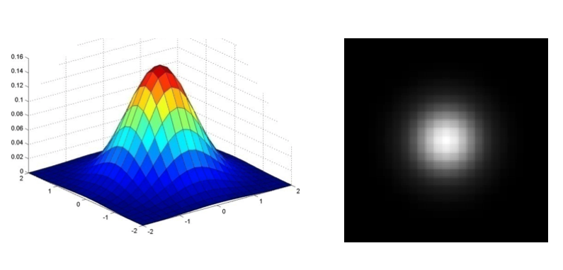
• We often use the following approximation of the Gaussian function

$$ \frac{1}{16} \left[ \begin{array}{ccc} 1 & 2 & 1 \\ 2 & 4 & 2 \\ 1 & 2 & 1 \end{array} \right] $$

• Gaussian function has infinite support, but discrete filters use finite kernels

Courtesy K. Grauman

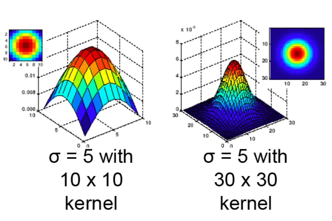
• Variance controls how broad or peaky the filter is

Courtesy K. Grauman

• Blurs the image, i.e., removes "high-frequency" components from the image (acts as low-pass filter)
• Convolution with itself is a Gaussian
• Convolving twice with Gaussian kernel of width $\sigma$ is the same as convolving once with kernel of width $\sigma \sqrt{2}$
• Applying a Gaussian filter with variance $\sigma_1$, followed by applying a Guassian filter with variance $\sigma_2$ is the same as applying once with Gaussian filter with variance $\sqrt{\sigma_1^2 + \sigma_2^2}$
• All values are positive
• Values sum to $1$? Why is this relevant?
• This size of the filter, plus its variance, determines the extent of smoothing

Exercise: applying 2D Gaussian & averaging kernels

Constuct a $15 \times 15$ Gaussian kernel of variance $7$ and blur the image I_gray. Also blur I_gray with a $23 \times 23$ averaging kernel. Compare the results.

Solution:

# %load solutions/linear-filtering/solution_04.py
# Blurring the image I_gray with two different kernels
width = 15

# Construct & apply 15x15 Gaussian kernel
gaussian_kernel = gaussian2d(7, width)
I_gauss = sp.signal.convolve2d(I_gray, gaussian_kernel, mode='same', boundary='fill')

# Construct & apply 15x15 averaging kernel
width = 15
averaging_kernel = np.ones([width, width])/(width*width)
I_ave = sp.signal.convolve2d(I_gray, averaging_kernel, mode='same', boundary='fill')

# Generate plots
plt.figure(figsize=(10,5))
plt.subplot(121)
plt.title('Gaussian Kernel')
plt.xticks([])
plt.yticks([])
plt.imshow(I_gauss[100:228,100:228], cmap='gray')
plt.subplot(122)
plt.xticks([])
plt.yticks([])
plt.title('Averaging (Box) Kernel')
plt.imshow(I_ave[100:228,100:228], cmap='gray');

Separability

A $n$-dimensional filter that can be expressed as an outer product of $n$ 1-dimensional filters is called a separable filter.

Example

$$ \left[ \begin{array}{ccc} 1 & 2 & 1 \\ 2 & 4 & 2 \\ 1 & 2 & 1 \end{array} \right] = \left[ \begin{array}{c} 1 \\ 2 \\ 1 \end{array} \right] \left[ \begin{array}{ccc} 1 & 2 & 1 \end{array} \right] $$

Convolutions with Separable Filters (in 2D)

• Step 1: Perform row-wise convolution with horizontal filter
• Step 2: Perform column-wise convolution of the result obtained in Step 1 with the vertical filter

Courtesy S. Fidler

Computational considerations

Where possible exploit separability to speed up convolutions. Say $w_k$ and $h_k$ denote kernel width and height, respectively, and $w$ and $h$ denote image width and height, respectively, then

• For separable filters: $\mathcal{O}(w_k \times w \times h) + \mathcal{O}(h_k \times w \times h)$

• For non-separable filters: $\mathcal{O}(w_k \times h_k \times w \times h)$

Separable Filters

• Use Singular Value Decomposition (SVD) to determine if a filter is separable. If only one singular value is non-zero then the filter is separable.

Recipe

(Step 1) Compute SVD, and check if only one singular value is non-zero

$$ F = \mathbf{U} \Sigma \mathbf{V}^T = \sum_i \sigma_i \mathbf{u}_i \mathbf{v}_i^T, $$

where $\Sigma = \mathrm{diag}(\sigma_i)$.

(Step 2). Vertical and horizontal filters are: $\sqrt{\sigma_1}\mathbf{u}_1$ and $\sqrt{\sigma_1}\mathbf{v}_1^T$

Code example

F = np.array([1,2,1,2,4,2,1,2,1]).reshape(3,3)
print('F =\n{}'.format(F))

print(np.linalg.matrix_rank(F))

u, s, vh = np.linalg.svd(F)
print(f'Singular values of F are: {s}')

print(u)
print(vh)

F =
[[1 2 1]
 [2 4 2]
 [1 2 1]]
1
Singular values of F are: [6.00000000e+00 4.71231182e-16 1.13655842e-48]
[[-0.40824829  0.91287093  0.        ]
 [-0.81649658 -0.36514837 -0.4472136 ]
 [-0.40824829 -0.18257419  0.89442719]]
[[-0.40824829 -0.81649658 -0.40824829]
 [-0.91287093  0.36514837  0.18257419]
 [-0.          0.4472136  -0.89442719]]

if s[~np.isclose(s, 0)].shape == (1,):
    print('Filter F_original is separable')
    ind = np.where(np.isclose(s, 0) == False)[0][0]
    s_1 = s[~np.isclose(s, ind)]
    fv = np.sqrt(s_1)*u[:,ind].reshape(3,1)
    fh = np.sqrt(s_1)*vh[ind,:].reshape(1,3)
    print('fv:\n {}'.format(fv))
    print('fh:\n {}'.format(fh))
    print('F_reconstructed:\n {}'.format(np.dot(fv, fh)))
else:
    print('Filter F is not separable')

Filter F_original is separable
fv:
 [[-1.]
 [-2.]
 [-1.]]
fh:
 [[-1. -2. -1.]]
F_reconstructed:
 [[1. 2. 1.]
 [2. 4. 2.]
 [1. 2. 1.]]

S = np.array([2,3,3,3,5,5,4,4,6]).reshape(3,3)

print('S*F: \n{}'.format(sp.signal.convolve2d(S, F, mode='valid')))

Sv = sp.signal.convolve2d(S, fv, mode='valid')
print('Sv=S*fv: \n{}'.format(Sv))
print('Sv*fh: \n{}'.format(sp.signal.convolve2d(Sv, fh, mode='valid')))

S*F: 
[[65]]
Sv=S*fv: 
[[-12. -17. -19.]]
Sv*fh: 
[[65.]]

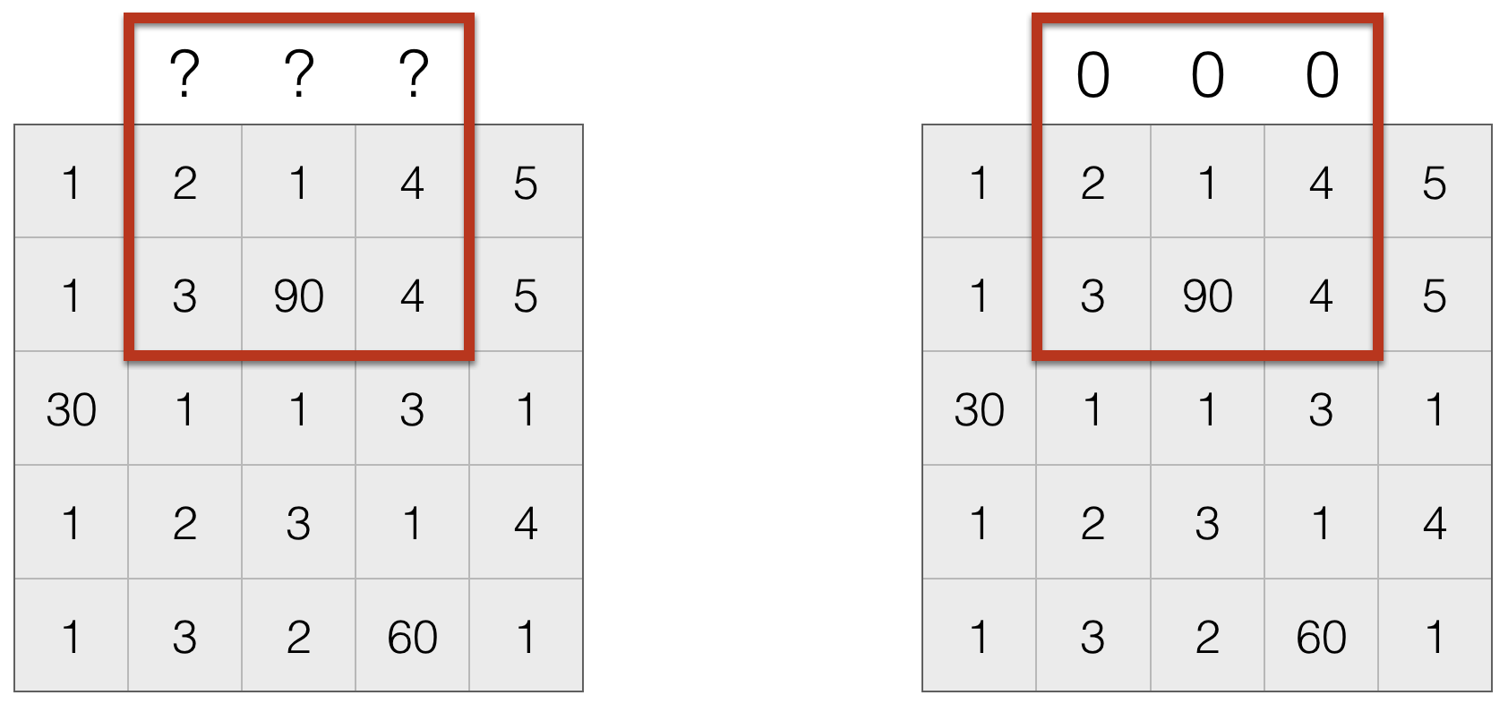
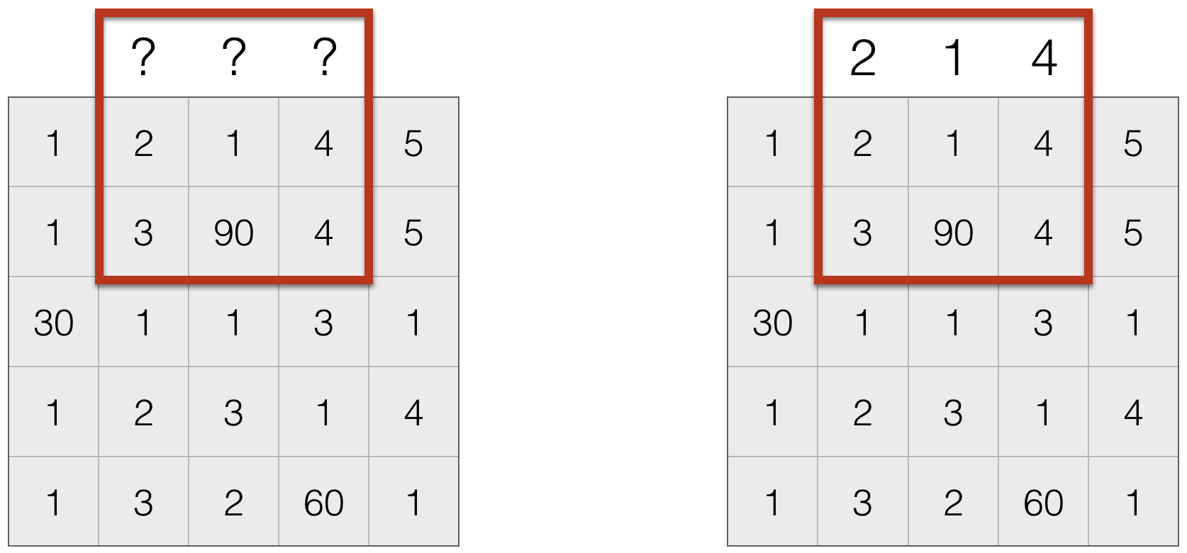
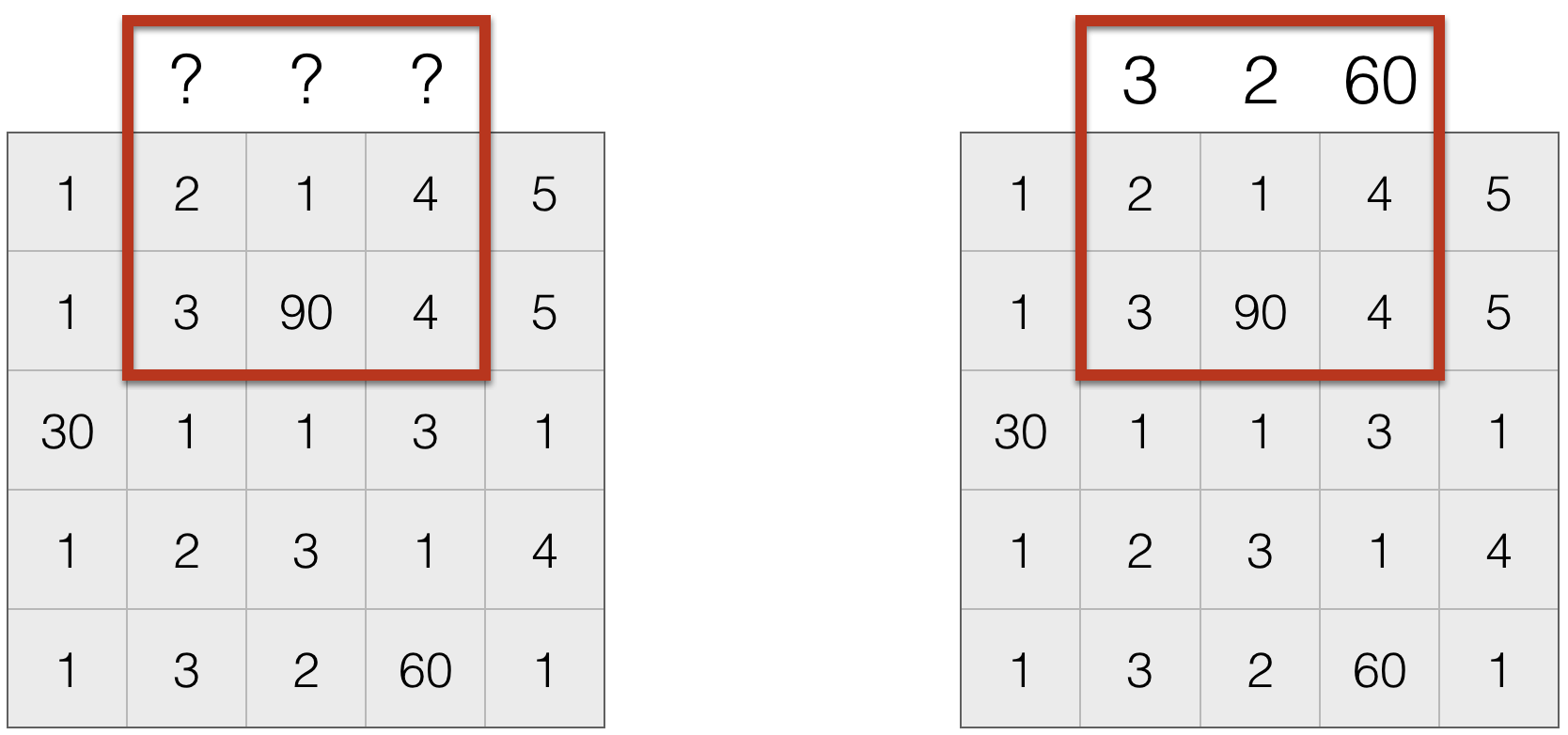
Dealing with Missing Values

• Set missing entries to a particular value, say $0$

• Repeat boundary entries

• Wrap around (this is useful to create an infinite domain)

• Do nothing. This is often not done, since the output size is not the same as the input size, which creates a host of practical issues.

Linear Filtering

• Linearity

$$ \mathtt{filter}(\alpha_1 f_1 + \alpha_2 f_2) = \alpha_1 \mathtt{filter}(f_1) + \alpha_2 \mathtt{filter}(f_2) $$

• Shift-invariance

$$ \mathtt{filter}(\mathtt{shift}(f)) = \mathtt{shift}(\mathtt{filter}(f)) $$

Any linear shift-invariant filter can be represented as a convolution.

Properties of Convolution

• Commulative: $a \ast b = b \ast a$
• Associative: $a \ast (b \ast c) = (a \ast b) \ast c$
• Distributes over addition: $a \ast (b+c) = a \ast b + a \ast c$
• Scalars factors out: $ka \ast b = a \ast kb = k (a \ast b)$
• Identity: $ a \ast e = a$, where $e$ is unit impulse

Relationship to Fourier Transform

The Fourier transform of two convolved signals is the element-wise (sometimes called Hadamard) product of their individual Fourier transforms:

$$ \mathcal{F}\left\{f \ast h\right\} = \mathcal{F}\left\{f\right\}\mathcal{F}\left\{h\right\}. $$

This also suggests that

$$ f \ast h = \mathcal{F}^{-1} \left\{ \mathcal{F}\left\{f\right\}\mathcal{F}\left\{h\right\} \right\}. $$

This is an important result. Why? Consider the relative complexity of compute $f \ast h$ using the Fourier transform trick ...

Note: there are many subtleties to what is meant by "the Fourier Transform," i.e., for signals on an unbounded, continuous domain (defined by integrals) or signals on a discrete bounded domain (the "discrete Fourier transform") and so on.

• For computational comparisons in Python, please consult The Convolution Theorem & Application Examples at dspillustrations.com
• An excellent technical reference is Briggs & Henson's The DFT: An Owner's Manual for the Discrete Fourier Transform that is very precise, comprehensive, and readable.

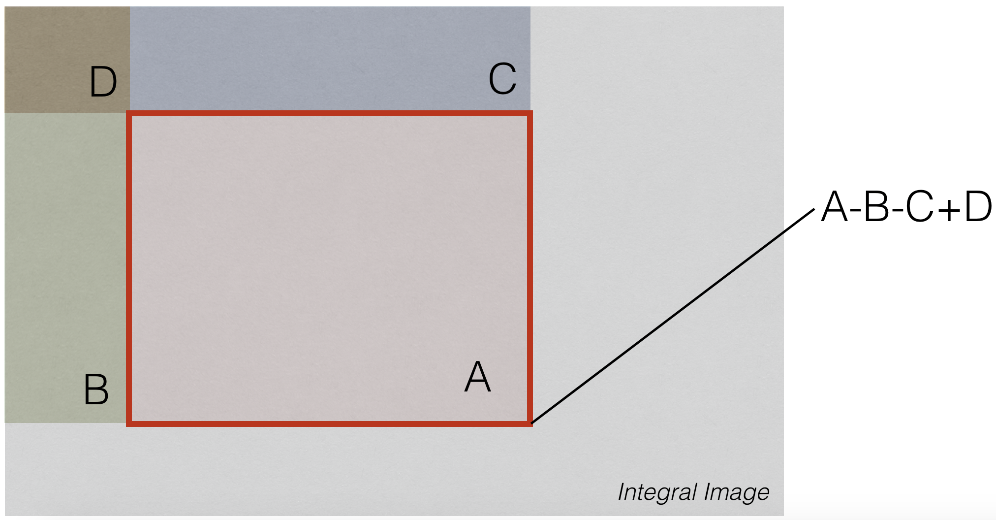
(Aside) Integral Images

Given an image $X[i,j]$, we compute the integral image as follows:

$$ S[m,n]=\sum_{i \le m} \sum_{j \le n} X[i,j] $$

(think of cumulative sums along both dimensions of an array).

X = np.array([1,2,3,-1,3,2,34,5,3,2,3,2,3,42,5,-3,1,4,98,3,1,2,3,2,5], dtype=np.float32).reshape(5,5)
print('X:\n {}'.format(X))
S = cv.integral(X)[1:,1:]
print('Integral image of X:\n {}'.format(S))

X:
 [[ 1.  2.  3. -1.  3.]
 [ 2. 34.  5.  3.  2.]
 [ 3.  2.  3. 42.  5.]
 [-3.  1.  4. 98.  3.]
 [ 1.  2.  3.  2.  5.]]
Integral image of X:
 [[  1.   3.   6.   5.   8.]
 [  3.  39.  47.  49.  54.]
 [  6.  44.  55.  99. 109.]
 [  3.  42.  57. 199. 212.]
 [  4.  45.  63. 207. 225.]]

Uses of Integral Images

No matter the size of summing window, we can compute sum using 3 arithmetic operations