CSCI 3240U: Computer Vision I

Lab 8: Homography and Image Stitching

Faisal Z. Qureshi
Faculty of Science, Ontario Tech University
Oshawa ON Canada
http://vclab.science.ontariotechu.ca

Fall 2026

Copyright information

© Faisal Qureshi

License

This work is licensed under a Creative Commons Attribution-NonCommercial 4.0 International License.

About this notebook

Read lab8.md first. This notebook covers the front of the lab only. It loads the image pair, holds your correspondences, and draws them so you can check them. Everything after that is yours to write.

Section here	Handout
Load the pair	Data
Correspondences, typed in	Part 1, Tasks 1 and 2
Optional interactive point picker	Part 1, Tasks 1 and 2
Task 3 stub: estimate the homography	Part 1, Task 3
Task 4 stub: warp and stitch	Part 1, Task 4
Part 2 checklist	Part 2, Tasks 5 to 10

Cells marked TODO are yours. Everything else runs as shipped.

Why the point picker is optional

The picker that this notebook used to open with needed %matplotlib tk. That backend fails in JupyterLab and in Colab, so the notebook would not run at all for most of the class. The default path now needs no interactive backend: you type your picked coordinates into two lists. The picker is still here, one section further down, guarded by a flag. Turn it on only if you run this notebook on a desktop Jupyter with %matplotlib tk, or locally with %matplotlib widget after installing ipympl. Neither works in Colab.

Any tool that reports pixel coordinates will do for the default path. Preview, GIMP and the Windows Photos app all show the cursor position, and so does the Matplotlib figure window when you run this notebook on your own machine.

Setup

import os

import cv2
import numpy as np
import matplotlib
import matplotlib.pyplot as plt

%matplotlib inline

print('OpenCV    ', cv2.__version__)
print('NumPy     ', np.__version__)
print('Matplotlib', matplotlib.__version__)

Helper code

Nothing below is graded. These helpers load images, display them, and draw labelled points. Read them before you use them.

Two conventions matter and they are easy to mix up.

• OpenCV point coordinates are (x, y), that is (column, row).
• NumPy array indices are [row, column].

Every point array in this notebook is (N, 2) holding (x, y), in float.

DATA_FOLDER = '.'


def load_rgb(filename):
    """Read an image and return it as RGB, ready for plt.imshow.

    cv2.imread gives you BGR.  Passing that straight to plt.imshow swaps red and
    blue, which is the classic first bug of every OpenCV lab.  The version of
    this notebook shipped before Fall 2026 had exactly that bug.
    """
    path = os.path.join(DATA_FOLDER, filename)
    bgr = cv2.imread(path)
    if bgr is None:
        raise FileNotFoundError(
            path + '\n'
            'Both images ship beside this notebook.  On Colab, upload '
            '1-left.jpeg and 1-right.jpeg into the working directory, or set '
            'DATA_FOLDER to wherever you put them.')
    return cv2.cvtColor(bgr, cv2.COLOR_BGR2RGB)


def show(img, title=None, size=(10, 10), cmap=None):
    """Display one image.  Pass an RGB array, not a BGR one."""
    plt.figure(figsize=size)
    if title:
        plt.title(title)
    if img.ndim == 2 and cmap is None:
        cmap = 'gray'
    plt.imshow(img, cmap=cmap)
    plt.axis('off')
    plt.show()


def show_pair(img_a, img_b, title_a='', title_b='', size=(18, 8)):
    """Display two RGB images side by side."""
    plt.figure(figsize=size)
    for i, (img, title) in enumerate([(img_a, title_a), (img_b, title_b)]):
        plt.subplot(1, 2, i + 1)
        plt.title(title)
        plt.imshow(img)
        plt.axis('off')
    plt.tight_layout()
    plt.show()


def draw_points(img, pts, colour=(255, 0, 0), radius=None, thickness=None,
                label=True):
    """Draw numbered circles on a copy of an RGB image.

    cv2.circle needs integer pixel coordinates.  Handing it NumPy floats raises
    a TypeError in OpenCV 4.10 and later, so round and cast here.
    """
    out = img.copy()
    h, w = out.shape[:2]
    if radius is None:
        radius = max(4, int(round(0.006 * max(h, w))))
    if thickness is None:
        thickness = max(2, radius // 3)
    for i, (x, y) in enumerate(np.asarray(pts, dtype=np.float64)):
        centre = (int(round(x)), int(round(y)))
        cv2.circle(out, centre, radius, colour, thickness)
        if label:
            cv2.putText(out, str(i), (centre[0] + radius, centre[1] - radius),
                        cv2.FONT_HERSHEY_SIMPLEX, radius / 12.0, colour,
                        thickness)
    return out

The image pair

1-left.jpeg and 1-right.jpeg are 4032 by 3024 pixels each. Full resolution is slow and wastes memory, and a Colab session will not thank you for a warped canvas of that size, so everything below works on a scaled copy.

SCALE sets the working resolution. Keep your correspondences in full resolution pixel coordinates and let the code scale them, so that your numbers stay valid when you change SCALE.

SCALE = 0.25   # working resolution; set to 1.0 for the full 4032 x 3024 images

left_full = load_rgb('1-left.jpeg')
right_full = load_rgb('1-right.jpeg')

left = cv2.resize(left_full, None, fx=SCALE, fy=SCALE,
                  interpolation=cv2.INTER_AREA)
right = cv2.resize(right_full, None, fx=SCALE, fy=SCALE,
                   interpolation=cv2.INTER_AREA)

print('full resolution   ', left_full.shape, right_full.shape)
print('working resolution', left.shape, right.shape)

show_pair(left, right, '1-left.jpeg', '1-right.jpeg')

Tasks 1 and 2: your correspondences

Fill in the two lists below. Each row is one point, written as [x, y] in full resolution pixels. Row $i$ of PTS_LEFT and row $i$ of PTS_RIGHT must name the same physical point in the scene. Order is everything: a pair of lists that disagree on order is the most common way to get a nonsensical homography, and the code cannot detect it for you.

The values below are an example, not an answer. They let the notebook run before you have picked anything. Replace them with your own picks, and pick more than four so that Part 1 can also look at the overdetermined case.

Where to pick, on this pair: the two photographs overlap over roughly the right quarter of the left image and the left quarter of the right image. Look at the window, the blind and the sill, the plant and its white pot, and the lamp arm. Nothing on the far left of the left image or the far right of the right image appears in both, so there is nothing there to pick.

Spread your points out. Four points crowded into one corner pin the homography there and let it run wild everywhere else. Depth matters too: most of the example points below sit on the plant, which is the nearest thing in the scene and therefore the worst affected by the camera moving between the two shots. Picking on the window and the sill instead is worth trying, and comparing the two homographies is worth a paragraph in your write-up.

# Example correspondences, in FULL RESOLUTION pixels. Replace with your own.
# Each row is [x, y]. Row i of PTS_LEFT matches row i of PTS_RIGHT.
PTS_LEFT = [
    [3097,  798],   # 0  on the blind, high in the overlap
    [3662, 1861],   # 1  leaf, upper part of the hanging plant
    [3321, 2234],   # 2  leaf against the window screen
    [3695, 2125],   # 3  leaf and stem above the white pot
    [3136, 2490],   # 4  leaf low on the left of the overlap
    [3966, 2576],   # 5  white pot, low on the right of the overlap
]

PTS_RIGHT = [
    [  90,  846],   # 0
    [ 705, 1841],   # 1
    [ 400, 2259],   # 2
    [ 761, 2097],   # 3
    [ 210, 2568],   # 4
    [1045, 2487],   # 5
]

pts_left = np.asarray(PTS_LEFT, dtype=np.float64) * SCALE
pts_right = np.asarray(PTS_RIGHT, dtype=np.float64) * SCALE

assert pts_left.shape == pts_right.shape, 'the two lists must be the same length'
assert pts_left.shape[0] >= 4, 'a homography needs at least four correspondences'
assert pts_left.ndim == 2 and pts_left.shape[1] == 2, 'each row must be [x, y]'

print(len(pts_left), 'correspondences at the working resolution')
print(np.round(np.hstack([pts_left, pts_right]), 1))

Check your correspondences before you use them

Look at the two figures below and read the numbers off. Point 3 on the left and point 3 on the right must sit on the same thing in the scene. Fix any that do not before you go any further. Debugging a homography whose input is wrong wastes an afternoon.

show_pair(draw_points(left, pts_left, colour=(255, 0, 0)),
          draw_points(right, pts_right, colour=(255, 0, 0)),
          'left: picked points', 'right: matching points')

Optional: the interactive point picker

This section needs an interactive Matplotlib backend and does not run in Colab. Skip it there and type your coordinates into the lists above.

To use it:

• on a desktop Jupyter, put %matplotlib tk in the cell below;
• locally in JupyterLab, pip install ipympl and use %matplotlib widget;
• then set RUN_PICKER = True and run the cell.

Under %matplotlib inline, which is what this notebook selects, the figure is a static image and no mouse events reach Python, so the picker collects nothing. The flag keeps that from looking like a bug.

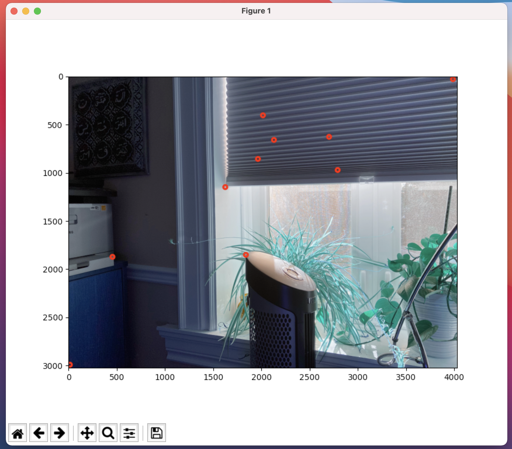
Click a point and the picker prints it, marks it, and appends it to picker.points. When you are done, run the cell after it to print your points in the format the lists above expect, then paste them in. That way your picks survive a restart, and the graders can see them.

RUN_PICKER = False   # set to True only with an interactive backend

# %matplotlib tk       # desktop Jupyter
# %matplotlib widget   # JupyterLab with ipympl installed


class PointPicker:
    """Collect (x, y) locations from mouse clicks on a Matplotlib image.

    The picked points are kept in self.points as (x, y) pairs in the
    coordinates of the array you passed in.  Multiply by 1 / SCALE to get back
    to full resolution pixels.
    """

    def __init__(self, imgplot, img, colour=(255, 0, 0), radius=8, thickness=3):
        self.imgplot = imgplot
        self.img = img.copy()
        self.colour = colour
        self.radius = radius
        self.thickness = thickness
        self.points = []
        self.cid = imgplot.figure.canvas.mpl_connect('button_press_event', self)

    def __call__(self, event):
        if event.inaxes != self.imgplot.axes:
            return
        if event.xdata is None or event.ydata is None:
            return
        x, y = float(event.xdata), float(event.ydata)
        self.points.append((x, y))
        print('%d: x=%.1f, y=%.1f' % (len(self.points) - 1, x, y))

        # cv2.circle needs integer coordinates; floats raise a TypeError.
        cv2.circle(self.img, (int(round(x)), int(round(y))), self.radius,
                   self.colour, self.thickness)
        self.imgplot.set_array(self.img)
        self.imgplot.figure.canvas.draw()

    def as_array(self, scale=1.0):
        """Return the picks as an (N, 2) float array, divided by scale."""
        return np.asarray(self.points, dtype=np.float64) / scale


if RUN_PICKER:
    picker_image = left        # or right
    fig = plt.figure(figsize=(10, 10))
    ax = fig.add_subplot(111)
    imgplot = ax.imshow(picker_image)   # RGB, so the colours are right
    picker = PointPicker(imgplot, picker_image)
    plt.show()
else:
    print('Picker off.  Type your coordinates into PTS_LEFT and PTS_RIGHT.')

# Run this after picking, then paste the output into the lists above.
if RUN_PICKER and picker.points:
    for x, y in picker.as_array(scale=SCALE):
        print('    [%4d, %4d],' % (round(x), round(y)))

Task 3: estimate the homography

From here on the code is yours. The handout allows you to start with cv2.findHomography so that you have something working, and then requires your own implementation. Write both and compare the two matrices.

Recall the shape of the problem. Each correspondence contributes two rows to $\mathbf{A}$, a homography has 8 degrees of freedom, and you solve $\mathbf{A}\mathbf{h} = \mathbf{0}$ with the SVD, exactly as in Lab 6. Then reshape $\mathbf{h}$ into a $3 \times 3$ matrix.

Decide which direction your $H$ maps, write it in the docstring, and keep it straight. Half of the failures in this lab are a matrix applied backwards.

def estimate_homography(src_pts, dst_pts):
    """Estimate H mapping src_pts to dst_pts.  Both are (N, 2) arrays of (x, y).

    Returns a 3x3 matrix.
    """
    # TODO (Task 3)
    #   1. build A, two rows per correspondence
    #   2. solve A h = 0 with the SVD
    #   3. reshape h to 3x3 and normalise
    raise NotImplementedError('Task 3: estimate_homography')

Task 4: warp and stitch

Warp one image into the frame of the other and put the two on one canvas.

Two details decide whether this works.

• Warp backwards. For each destination pixel, apply the inverse mapping to find where it came from in the source, then interpolate there. Forward warping scatters source pixels into the destination and leaves a lattice of holes. The handout warns about this and the warning is worth heeding.
• Size the canvas first. Map the four corners of the image you are warping into the destination frame. Their bounding box, unioned with the destination image, tells you how large the canvas must be and how far to translate everything so that nothing lands at a negative coordinate.

On this pair the two photographs overlap over about a quarter of their width, and the camera translated rather than rotated, so expect a visibly distorted result with ghosting on the near objects. That is the parallax the handout asks you to discuss, not a bug in your code. Crop the canvas before you display it if it comes out very large.

def warp_backward(img, H, out_shape):
    """Warp img into an out_shape canvas using backward mapping.

    out_shape is (height, width).  Returns an array of that shape.
    """
    # TODO (Task 4)
    #   1. build the grid of destination pixel coordinates
    #   2. map them into the source with the inverse of H
    #   3. interpolate the source at those locations, bilinear is expected
    #   4. leave destination pixels whose source falls outside the image alone
    raise NotImplementedError('Task 4: warp_backward')


def stitch(img_left, img_right, H):
    """Place both images on one canvas and return it."""
    # TODO (Task 4)
    #   1. map the corners of the warped image into the reference frame
    #   2. work out the canvas size and the translation that keeps it positive
    #   3. warp, then paste the reference image in
    raise NotImplementedError('Task 4: stitch')

Then: more than four points

Repeat Task 3 with more correspondences and report what changes. The handout asks you to show it, so show a figure or a table, not a sentence. Watch the smallest singular value of $\mathbf{A}$ as you add points, and say what it measures.

Part 2: doing it automatically

No starter code here. Tasks 5 to 10 are yours, and the handout lists them. The pieces you need already exist in earlier labs.

• Detect and describe with cv2.SIFT_create(). SIFT moved into the main OpenCV module in version 4.4. cv2.xfeatures2d.SIFT_create() is gone from opencv-python and raises an AttributeError.
• Match with cv2.BFMatcher and knnMatch, then apply the ratio test.
• Run RANSAC over the putative matches, as in Lab 6, and report the inlier count.
• Justify your iteration count from the inlier ratio you observed. Quoting a default of 1000 earns nothing.
• Show the no-RANSAC failure: least squares over every putative match, outliers included.

One warning about this particular pair. The overlap is small, the scene is indoors, and the blind fills much of the frame with a repeating pattern, so plain SIFT matching on it proposes many wrong matches and the inlier ratio comes out low. Report the ratio you measure and let it drive your iteration count. If your automatic result is poor here, say so and explain why, using the putative match figure as evidence. A pair of your own, shot by rotating in place, will behave much better.

Submission

Submit a single Jupyter notebook via Canvas. Run it top to bottom before you submit, so every figure and every number is visible in the file. Code that has not been executed cannot be marked.