Introduction

The goal of this lab is to find the points in an image that are worth paying attention to, and then to do two different things with them: follow them through time, and describe them so they can be recognised in another image.

The unifying object is the structure tensor \(M\). You will build it once in Part 1 to decide whether a point is a corner, and then discover in Part 2 that the same matrix, with the same eigenvalues, decides whether optical flow can be estimated there at all. Corner detection and the aperture problem turn out to be two readings of one statement — which is why Shi and Tomasi called their paper Good Features to Track.

This lab builds directly on the gradient machinery from Lab 4 and the pyramid from Lab 5. It feeds into Lab 8, where you will use these correspondences to estimate a homography.

Reading

Computer Vision: Algorithms and Applications (2nd ed.), Szeliski — Sec. 7.1.1–7.1.3, 7.1.5, 9.3.

Feature detectors, descriptors, matching and tracking; optical flow.

Data

Two sources, both supplied:

• Landmark images for Parts 1, 3 and 4 — local-features-construction-1.jpg, local-features-construction-2.jpg, cn-tower-1.jpg, cn-tower-2.jpg, eiffel-tower.jpeg and the two corrupted CN Tower images.
• Video for Part 2 — traffic-short.mp4, the fixed-camera highway footage you already used in Lab 1.

Part 1: Corner detection

Starter code is provided in corner-detection-starter.ipynb [html].

Task 1. Find interest points using the Harris corner detector.

Task 2. Find interest points using the Shi-Tomasi detector.

Task 3. Display both sets of interest points on the same image and comment on the differences.

Task 4. Rotate the image by 30 degrees and re-run both detectors. Do the same physical points get detected? Quantify this rather than eyeballing it — for example, map the detections from the rotated image back into the original frame and count how many land within a few pixels of an original detection.

Recall that both detectors are built from the structure tensor \[ M = \sum_{(x,y) \in W} w(x,y) \left[ \begin{array}{cc} I_x^2 & I_x I_y \\ I_x I_y & I_y^2 \end{array} \right], \] and differ only in how they turn the eigenvalues of \(M\) into a corner score. You already know how to compute \(I_x\) and \(I_y\) from Lab 4.

Part 2: Optical flow and tracking

You have just built \(M\) to answer “is this a corner?”. Now you will use it to answer a different question: “can I tell how this point moved?”

The data

This part uses traffic-short.mp4, the highway footage from Lab 1. The camera is static, which matters: anything that moves in the image is something that moved in the world.

In Lab 1 you subtracted consecutive frames and called it a crude motion detector. This is where we do it properly.

Task 5: derive it

Assume brightness constancy — a small patch keeps its intensity as it moves: \[ I(x,y,t) = I(x + u,\; y + v,\; t + 1). \]

Take the first-order Taylor expansion and show that this gives \[ I_x u + I_y v + I_t = 0 \] for each pixel, where \(I_t\) is the temporal derivative.

One equation, two unknowns. State clearly what this means for a single pixel: you can recover the component of motion along the gradient, and nothing about the component perpendicular to it. This is the aperture problem.

Task 6: solve it over a window

Lucas-Kanade assumes the flow is constant over a small window \(W\), giving one equation per pixel in \(W\) and hence an overdetermined system. Show that the least-squares solution is \[ \left[\begin{array}{c} u \\ v \end{array}\right] = -M^{-1} \left[\begin{array}{c} \sum I_x I_t \\ \sum I_y I_t \end{array}\right], \] where \(M\) is exactly the structure tensor you built in Part 1.

Implement Lucas-Kanade for a single point. You will need \(I_t\), which is just the difference between the two frames.

Task 7: the aperture problem, measured

Pick three patches in one frame: one on a corner, one on a long straight edge (a lane marking or the guardrail is ideal), and one on a textureless region (the sky, or open snow).

For each, report the two eigenvalues of \(M\), and their ratio.

Then answer:

• Which patches give an invertible \(M\)? Which give a well-conditioned one?
• Relate each case to what you can and cannot recover about the motion.
• Compare against the Harris and Shi-Tomasi scores you computed in Part 1 for the same patches. They should rank the patches the same way. Explain why that is not a coincidence.

Task 8: track

Detect Shi-Tomasi corners in one frame and use your Lucas-Kanade to follow them into the next. Draw the flow vectors on the image.

Most of your corners will barely move — they are on the road surface, the barrier and the bridge, which are stationary. That is correct. Use the flow magnitude to separate the moving vehicles from the static background, and show the result.

Report what fraction of your detected corners are moving. On this footage it will be a small minority.

Task 9: where single-scale Lucas-Kanade breaks

Vehicles close to the camera move a long way between frames — far more than a \(21\times21\) window can see. Lucas-Kanade is derived from a first-order Taylor expansion, so it is only valid for small displacements.

1. Find a patch on a vehicle in the near lane and measure its true displacement independently, using template matching (cv.matchTemplate) over a generous search region. This is your reference.
2. Run your single-window Lucas-Kanade on the same patch. Compare.
3. Now run it coarse-to-fine: estimate the flow at a coarse level of the Gaussian pyramid you built in Lab 5, upscale that estimate by 2, use it to warp the window, and refine at the next level down. Compare again.

Report all three numbers. You should find that single-scale Lucas-Kanade substantially underestimates large motion while the pyramidal version tracks it, and that both agree on slow-moving distant vehicles.

Explain in one paragraph why a pyramid fixes this, in terms of how far a point moves in pixels at each level.

Task 10: honest failure cases

Find and show one example of each:

• a point where flow is estimated confidently but wrongly, because the local structure is repetitive (the guardrail posts are a good hunting ground);
• a point where no flow can be estimated at all, and say which eigenvalue of \(M\) told you so in advance.

You may use cv.calcOpticalFlowPyrLK to check your own implementation, and you should say whether the two agree.

Part 3: A SIFT-like local descriptor

Starter code is provided in sift-like-descriptor.ipynb [html].

You will build a 128-dimensional rotation-invariant descriptor by hand. Use local-features-construction-2.jpg to test your code.

Task 11

Complete the steps needed to compute the rotation invariant descriptor:

• Take a \(16 \times 16\) patch around the interest point.
• Compute gradient magnitudes and orientations in the patch.
• Weight the gradient magnitudes by a Gaussian centred on the patch.
• Find the dominant orientation of the patch, and rotate all gradient orientations so that the dominant orientation points to zero. This is the step that buys you rotation invariance.
• Divide the patch into a \(4 \times 4\) grid of cells. For each cell, build an 8-bin orientation histogram weighted by gradient magnitude.
• Concatenate the 16 histograms into a single \(16 \times 8 = 128\) dimensional vector and normalize it.

Task 12

Combine your code into the following method:

descriptor, I_patch, grad_patch, grad_patch_weighted, grad_color_patch = my_local_descriptor(img, r, c)

This method takes an image img and a row r and column c location, and returns a 128-dimensional descriptor. It also returns four \(16 \times 16\) patches around the (r,c) location: I_patch is the image intensity patch, grad_patch is the gradient magnitudes, grad_patch_weighted is the weighted gradient magnitudes, and grad_color_patch is the colourized gradient magnitudes.

Task 13

Compute descriptors at corresponding locations in local-features-construction-1.jpg and local-features-construction-2.jpg, and compare them. Are the two descriptors similar? Now compute a descriptor at an unrelated location and compare again. Report the distances.

Part 4 (optional): Deciding whether two images match

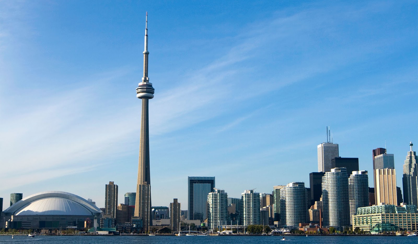
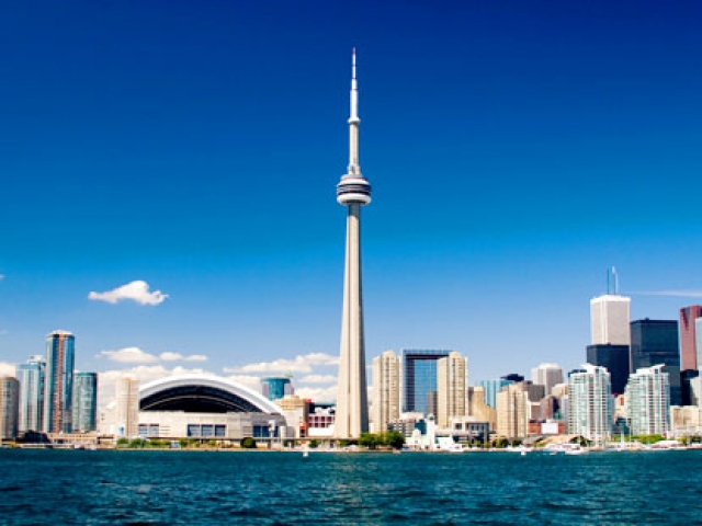
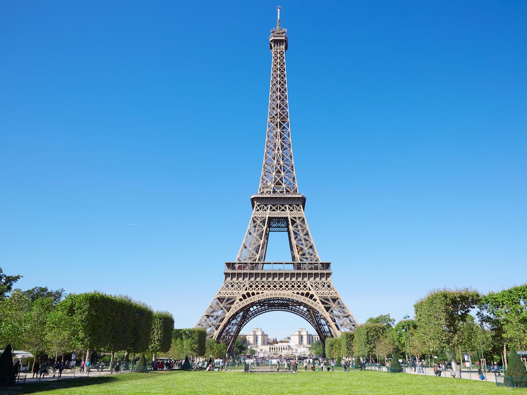
Given a triplet of images \((A, B, C)\), use local features to decide which of the three pairs — \((A,B)\), \((A,C)\), \((B,C)\) — is the closest. For example, if your triplet contains two images of the CN Tower and one of the Eiffel Tower, your algorithm should return the pair containing the two CN Tower images.

1. Construct a triplet from cn-tower-1.jpg, cn-tower-2.jpg and eiffel-tower.jpeg.
2. Compute keypoints and descriptors for each image. You may use OpenCV’s SIFT or KAZE implementation here — Part 2 was where you had to build it yourself.
3. Match descriptors between image pairs and record the fraction of “good” matches. You will need to decide what makes a match “good”; the ratio test is a reasonable place to start.
4. Use the good-match counts to decide which two images are closest.
5. Repeat using the corrupted versions, cn-tower-1-corrupted.jpg and cn-tower-2-corrupted.jpg. Does your method still pick the right pair?

Bonus

Test your code on images from the Image Matching Challenge.

Deliverables

Your notebook must contain the following.

• Harris and Shi-Tomasi detections, displayed and compared, with non-maximum suppression applied.
• Rotation repeatability quantified by location, not by detection count.
• The Lucas-Kanade derivation, ending at \(M\mathbf{u} = -\mathbf{b}\).
• An eigenvalue table for a corner, an edge and a textureless patch, with the ranking compared against your Part 1 corner scores.
• Flow vectors drawn on a frame, a moving/static segmentation, and the fraction of corners that actually move.
• A three-way displacement comparison — template-matching reference, single-scale Lucas-Kanade, and pyramidal Lucas-Kanade — on a fast-moving vehicle, with an explanation of why the pyramid helps.
• Two failure cases: one confident-but-wrong, one where no flow is recoverable, with the eigenvalue that predicted it.
• my_local_descriptor returning a 128-D descriptor and the four patches, with the orientation-normalisation step actually applied.
• Descriptor distances at corresponding and unrelated points, so the separation is visible.

Submission

Via Canvas. Please submit a single executed Jupyter notebook — one that has been run top to bottom, so that every figure and number listed above is visible in the submitted file. Code that has not been executed cannot be marked.

Parting thoughts

• Part 1 asks you to check rotation robustness, and Part 2 asks you to build in rotation invariance. These are two different things. Be clear in your write-up about which property you are testing.
• A descriptor is only useful if similar things are close together and dissimilar things are far apart. Reporting one distance tells me nothing; reporting the distribution of distances tells me everything.
• Matching produces plenty of wrong correspondences even on easy image pairs. Lab 8 is where we deal with that properly.