Introduction

The goal of this lab is to build Gaussian and Laplacian pyramids, and then to use them to answer a practical question: at what scale should you look for a road boundary?

In Lab 4 you produced an edge map at full resolution and scored it against ground truth. You almost certainly found that fine detail — kerb texture, tyre marks, cracks, shadows — generated edge pixels that had nothing to do with the road boundary. Scale is one of the tools for dealing with that, and in Lab 6 you will need to decide which resolution to run your line fitting at.

Reading

Computer Vision: Algorithms and Applications (2nd ed.), Szeliski — Sec. 3.5.

Pyramids and wavelets — interpolation, decimation, and multi-resolution representations.

Data

This lab continues with the KITTI Road benchmark from Lab 4. See Getting the KITTI data if you have not set it up yet. You will also reuse your gradient and edge code from Lab 4.

A note on loading the data

Parsing KITTI’s calibration format and decoding its colour-coded ground truth is plumbing, not computer vision, and debugging it eats time you should be spending on the lab. A small helper module is provided: kitti.py.

import kitti

ds  = kitti.Dataset("path/to/data_road")     # point at the extracted folder
img = ds.image("um_000032")                  # left image, RGB uint8
cal = ds.calib("um_000032")                  # cal.K, cal.fx, cal.baseline, ...
pos, valid = ds.ground_truth("um_000032")    # boolean masks

It deliberately does not implement anything you are asked to write yourself — no edge detection, no region of interest, no scoring. You are free to ignore it and do your own file handling if you prefer.

Part 1: Building the pyramids

Task 1

Implement downsampling and upsampling:

def pyr_down(image):    # blur, then subsample by 2
def pyr_up(image):      # upsample by 2, then blur

Reuse the Gaussian filtering code from Lab 3.

Note the order of operations in pyr_down. Blurring before subsampling is not optional. Show what happens if you subsample a KITTI image without blurring first, and explain the artifacts. Lane markings and railings are an excellent place to look for them.

Task 2

Construct a Gaussian pyramid with at least 5 levels and display all of them.

Task 3

Construct a Laplacian pyramid. Recall that level \(i\) is \[ L_i = G_i - \mathrm{pyrUp}(G_{i+1}), \] where \(G_i\) is level \(i\) of the Gaussian pyramid, and the last Laplacian level is the last Gaussian level.

Task 4

Show that your Laplacian pyramid is invertible. Reconstruct the original image from the pyramid and report the maximum absolute difference against the original. It should be very close to zero. If it is not, your pyr_up and pyr_down are inconsistent — fix that before continuing, because Part 2 depends on it.

Part 2: Scale and the road

Task 5: edges across scale

Take your edge detector from Lab 4 and run it at every level of the Gaussian pyramid of a KITTI image. Display the resulting edge maps side by side, each upsampled back to the original resolution so they can be compared.

Describe what happens as you go up the pyramid. Which edges survive? Which disappear first?

Task 6: which scale is best?

Score each of those edge maps against the ground-truth road boundary using the recall and selectivity measures you built in Lab 4 (tolerance \(\tau = 3\) pixels, measured at full resolution).

Plot recall and selectivity against pyramid level, averaged over at least 10 images. Also record the number of pixels you actually processed at each level.

Then answer:

• How much recall do you lose going from level 0 to level 1? How many fewer pixels did you process to get it? Is that a good trade?
• At what level does recall start to fall off sharply? Relate this to the width in pixels of the structures you are trying to keep — a lane marking is only a few pixels across at full resolution, so how many levels can it survive?
• Which level would you run your Lab 6 line fitting at, and why? Note that fitting a line does not need the fine detail that locating an edge does.

Task 7: coarse-to-fine

Coarse levels are cheap; fine levels are accurate. Sketch — in code or in clear pseudocode — how you would use a coarse level to restrict where you search at a finer level, rather than processing the whole fine image.

Estimate the speed-up this would give you and state the assumption your estimate depends on.

Part 3 (optional): Hybrid images

If you have time, this is the classic demonstration of what a Laplacian pyramid buys you.

A hybrid image is a static image that changes with viewing distance: up close you see one picture, from across the room you see another. The human visual system picks up high spatial frequencies close up and cannot resolve them from a distance, so only the low-frequency content survives at range.

Given two images A and B:

• Construct the Laplacian pyramid of A.
• Construct the Laplacian pyramid of B.
• Build a new pyramid taking some levels from A and the rest from B.
• Reconstruct the image from this new pyramid.

The two images must be roughly aligned — the eyes in one face should sit approximately where the eyes in the other do. Crop and resize as needed.

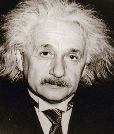
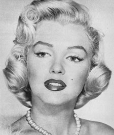
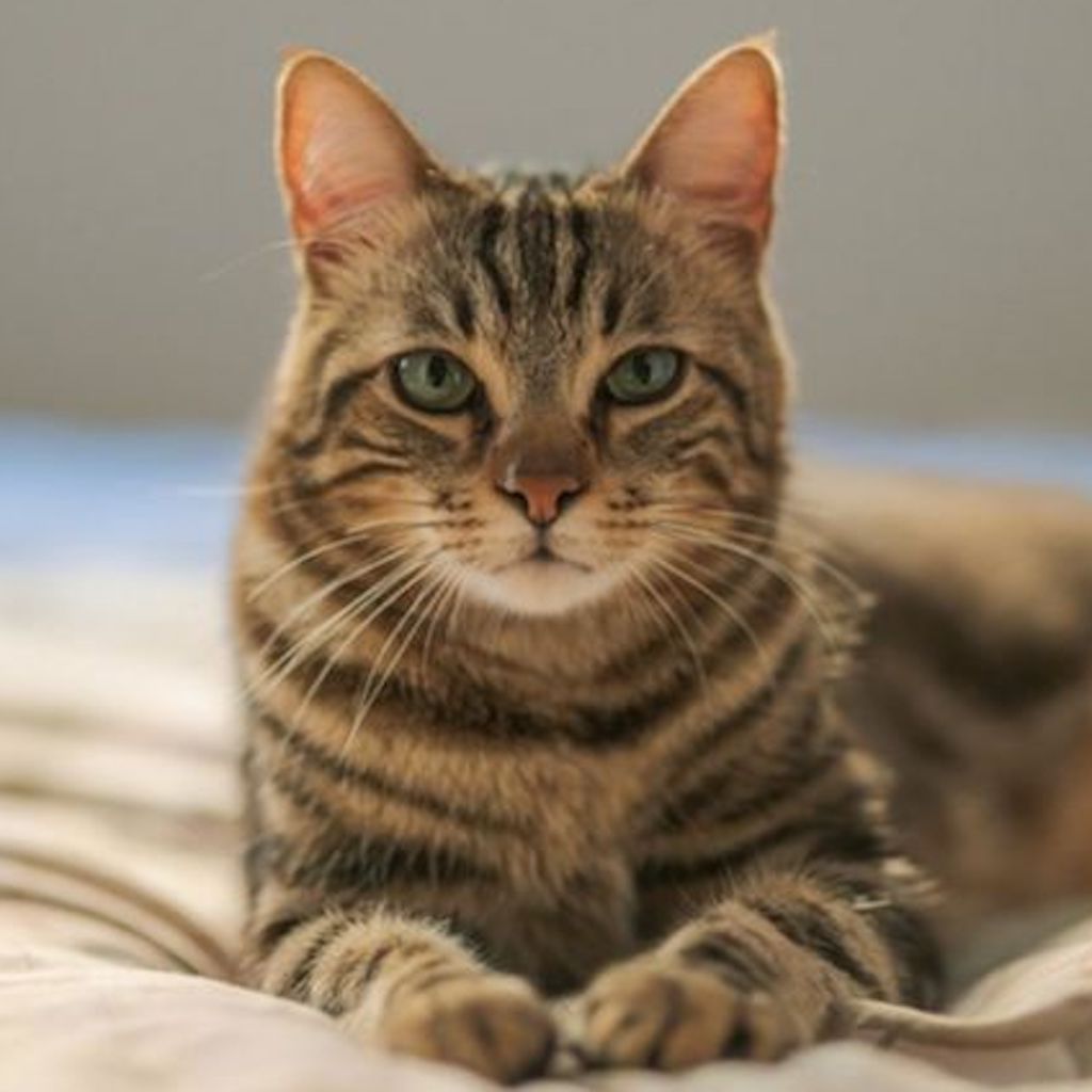
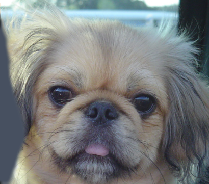
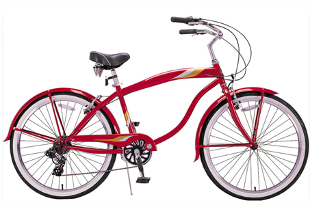
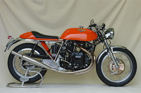
Provided pairs: einstein.bmp/marilyn.bmp, cat.jpg/dog.bmp, and bicycle.bmp/motorcycle.bmp.

Show your result at full size and at \(1/4\) and \(1/8\) scale so the effect is visible in the notebook, and try at least two different cut-off levels. Which image should supply the low frequencies? There is no single right answer, but there is definitely a wrong one — try it both ways round.

Deliverables

Your notebook must contain the following.

• pyr_down and pyr_up, and a cropped figure showing subsampling without pre-blurring, with the artifacts explained.
• A Gaussian pyramid of at least 5 levels and a Laplacian pyramid, both displayed.
• The reconstruction error from the invertibility check, as a number.
• Edge maps computed at every pyramid level, upsampled to full resolution and shown side by side.
• A plot of recall and selectivity against pyramid level, averaged over at least 10 images, together with the pixel count processed at each level.
• Answers on the level 0 → 1 trade, where recall falls off and why, and which level you would hand to Lab 6.
• Coarse-to-fine pseudocode, a speed-up estimate, and the assumption it rests on.

Submission

Via Canvas. Please submit a single executed Jupyter notebook — one that has been run top to bottom, so that every figure and number listed above is visible in the submitted file. Code that has not been executed cannot be marked.

Parting thoughts

• Implement pyr_down and pyr_up yourself. Compare against cv.pyrDown and cv.pyrUp once yours works, but do not start there.
• KITTI images are roughly \(1242 \times 375\) — much wider than they are tall. After four levels you have very little vertical resolution left. Say how many levels are actually useful for these images and why.
• When you upsample an edge map for comparison, use nearest-neighbour interpolation, not bilinear. Interpolating a binary mask gives you grey values that are neither edge nor not-edge.
• Aliasing is the whole point of Task 1. If you have never seen a badly subsampled image before, look closely at the lane markings — they will break into dashes that were never there.