Introduction

The goal of this lab is to implement linear filtering from the ground up, and then to understand what makes a filter fast. You will write your own convolution, use it to blur an image, and then measure how badly your implementation loses to a library implementation — and work out why.

Convolution is the single most reused operation in this course. Everything in Lab 4 (gradients and edges), Lab 5 (pyramids) and Lab 10 (convolutional networks) is built on what you write today, so it is worth getting right.

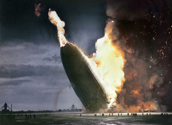
Use hindenburg.jpg as your test image.

Do not use cv.blur, cv.GaussianBlur, cv.filter2D or scipy.ndimage.convolve for Parts 1–3. The point of this lab is to build the thing, not to call it. You will use them in Part 4 for comparison.

Reading

Computer Vision: Algorithms and Applications (2nd ed.), Szeliski — Sec. 3.2.

Linear filtering, including separable filtering (Sec. 3.2.1).

Data

A single image, hindenburg.jpg, supplied beside this handout. No download is required.

Part 1: Writing your own convolution

Task 1

Implement

def apply_filter_to_patch(patch, filter):

which applies an \(h \times w\) filter to an \(h \times w\) patch and returns a scalar value.

Task 2

Use the method above to implement full-image linear filtering:

def apply_filter_to_image(image, filter):

which returns an image. Internally this method must use your own apply_filter_to_patch method.

Ignoring the boundary is acceptable, but state clearly in your notebook what your function does at the edges of the image and what size of output it returns. Boundary handling is not a detail — in Lab 4 it will produce a spurious “edge” all the way around your image if you get it wrong.

Task 3

Construct and visualize an \(11 \times 11\) Gaussian kernel for \(\sigma = [1, 3, 5]\). Convolve the hindenburg image with each of the three kernels and show the results.

Recall that a 2D Gaussian is \[ G(x,y) = \frac{1}{2\pi\sigma^2} e^{-\frac{x^2+y^2}{2\sigma^2}}. \]

Normalize your kernel so that its entries sum to \(1\). Show what the image looks like if you don’t, and explain what went wrong.

Task 4

An \(11 \times 11\) kernel with \(\sigma = 5\) is a poor pairing. Explain why, and state a sensible rule of thumb relating kernel size to \(\sigma\). Support your answer with a plot of the kernel values.

Part 2: Separability

Task 5

Consider the following kernel: \[ \left[ \begin{array}{ccc} 7 & 34 & 3 \\ 0 & 0 & 0 \\ -7 & -34 & -3 \end{array} \right] \]

Confirm that it is separable. Convolve the hindenburg image with this kernel directly. Next, exploit separability — convolve with the two 1D kernels in sequence instead — and convolve the image again. Are the two results the same, or different? Explain what you observe.

Hint: a matrix is separable if and only if it has rank 1. The SVD will tell you this, and it will also hand you the two 1D kernels.

Task 6

Is your Gaussian kernel from Task 3 separable? If so, write a separable version of the Gaussian blur.

Part 3: Filtering at several scales

Blur the hindenburg image with your Gaussian for \(\sigma \in \{1, 2, 4, 8, 16\}\) and display the results side by side.

Describe what disappears first as \(\sigma\) grows, and what survives longest. Relate your answer to spatial frequency. Keep these images — you will compare them against the pyramid representation in Lab 5.

Part 4: How slow is your convolution?

Now bring in the library implementations.

Task 7

Time the following, for square kernels of half-width \(1, 2, 4, 8, 16\):

1. Your apply_filter_to_image with a 2D Gaussian.
2. Your separable Gaussian from Task 6.
3. OpenCV’s GaussianBlur.

Present the timings in a table and as a plot, with kernel half-width on the horizontal axis and time on the vertical.

Task 8

Answer the following, with evidence from your measurements:

• How does the cost of your 2D convolution grow with kernel half-width? How does the separable version grow? Do your measurements match the theory?
• How much faster is OpenCV than your separable version? Separability alone does not explain the whole gap — suggest what else OpenCV is doing.
• Is the box (averaging) filter faster or slower than the Gaussian at the same kernel size? Why?

Deliverables

Your notebook must contain the following.

• apply_filter_to_patch and apply_filter_to_image, plus a statement of what your code does at the image boundary and what size output it returns.
• Gaussian kernels for \(\sigma = 1, 3, 5\), visualised, with the blurred results.
• The un-normalised result, with an explanation of what went wrong.
• Your kernel-size rule of thumb, supported by a plot of the kernel values.
• Evidence that the Task 5 kernel is separable (rank or SVD), and a comparison of the direct and separable results.
• The multi-scale blur for \(\sigma \in \{1,2,4,8,16\}\).
• A timing table and plot covering all three implementations at five kernel sizes, with the Task 8 answers.

Submission

Via Canvas. Please submit a single executed Jupyter notebook — one that has been run top to bottom, so that every figure and number listed above is visible in the submitted file. Code that has not been executed cannot be marked.

Parting thoughts

• Record your timings in a pandas dataframe. It makes the analysis and the plotting far easier, and you will want the same habit in Lab 4.
• Time each configuration more than once and report the median. A single measurement on a laptop is mostly noise.
• Watch your data types. If you convolve an 8-bit unsigned image you will get wraparound on any value that leaves the \([0,255]\) range. Convert to float first, and convert back only for display.
• A box filter is separable too. It is also computable in time independent of kernel size using a running sum — worth a look if you finish early.