Introduction

The goal of this lab is to take the pinhole camera model off the whiteboard and point it at a real camera.

You will read the actual calibration of the camera that recorded the KITTI dataset, use it to project 3D points into the image, and then run the process backwards — taking a pixel and recovering where in the world it came from. By the end you will be able to look at a photograph of a road and say, in metres, how far away things are.

Everything here is the projection equation \[ \tilde{\mathbf{x}} = P\,\tilde{\mathbf{X}}, \qquad P = K \left[\begin{array}{cc} R & \mathbf{t}\end{array}\right], \] used forwards and then backwards.

Reading

Computer Vision: Algorithms and Applications (2nd ed.), Szeliski — Sec. 2.1.4, 2.1.5, 11.1.

3D to 2D projections, lens distortions, and geometric intrinsic calibration.

Data

The KITTI Road benchmark. See Getting the KITTI data — --left-only is enough for this lab. You can also start immediately with the three sample scenes in ../data/kitti-samples, each of which has an image and its calibration file.

A note on loading the data

Parsing KITTI’s calibration format and decoding its colour-coded ground truth is plumbing, not computer vision, and debugging it eats time you should be spending on the lab. A small helper module is provided: kitti.py.

import kitti

ds  = kitti.Dataset("path/to/data_road")     # point at the extracted folder
img = ds.image("um_000032")                  # left image, RGB uint8
cal = ds.calib("um_000032")                  # cal.K, cal.fx, cal.baseline, ...
pos, valid = ds.ground_truth("um_000032")    # boolean masks

It deliberately does not implement anything you are asked to write yourself — no edge detection, no region of interest, no scoring. You are free to ignore it and do your own file handling if you prefer.

Part 1: Reading a real camera matrix

Each calib/*.txt contains four projection matrices. P0 and P1 are the grey cameras; P2 is the left colour camera, which took the images you will work with, and P3 is the right colour camera. Each is \(3\times4\).

Task 1

Parse P2 for one scene. Split it as \[ P_2 = \left[\begin{array}{cc} K & K\mathbf{t}\end{array}\right], \] so \(K\) is the leftmost \(3\times3\) block. Report:

• the focal lengths \(f_x\) and \(f_y\), in pixels
• the principal point \((c_x, c_y)\), in pixels
• the skew

Task 2: sanity checks

A camera matrix you have parsed correctly should pass these:

• \(f_x\) and \(f_y\) should be equal, because the pixels are square.
• The skew should be zero. Real cameras essentially never have skew; a non-zero value means you have mis-parsed.
• \((c_x, c_y)\) should sit near the middle of the image. Compare against the image dimensions and comment on any discrepancy — KITTI images are cropped after rectification, so it is not exactly centred.

Report all three checks. Then repeat for a second scene: is the calibration the same across scenes, and why would that be?

Task 3: what the focal length means

\(f_x\) is a focal length expressed in pixels, not millimetres. Show that the horizontal field of view is \[ \text{FOV}_x = 2\arctan\!\left(\frac{W}{2f_x}\right), \] and compute it for this camera. Does the number you get look consistent with the images you are seeing?

Part 2: Projecting into the image

The car carried a laser scanner and the calibration includes Tr_cam_to_road, the transform from camera coordinates to a plane fitted to the road surface. The last column’s \(y\) component gives the height of the camera above the road, which is the one piece of world knowledge you need.

Task 4

Extract the camera height \(h\) from Tr_cam_to_road. You should get something close to the height of a camera mounted on a car — if you get 0.02 or 160, you have picked the wrong element.

Task 5: project a point

In camera coordinates, \(+Z\) points forward along the optical axis, \(+X\) to the right and \(+Y\) down. So a point on the road surface \(Z\) metres ahead and \(X\) metres to the side is \((X,\ h,\ Z)\).

Write

def project(P, X):        # X is a 3-vector in camera coordinates
    ...                   # returns (u, v) in pixels

remembering to divide by the third homogeneous coordinate. Project the points \((0, h, Z)\) for \(Z = 5, 10, 20, 50\) m and report the pixel coordinates.

Task 6: draw a grid on the road

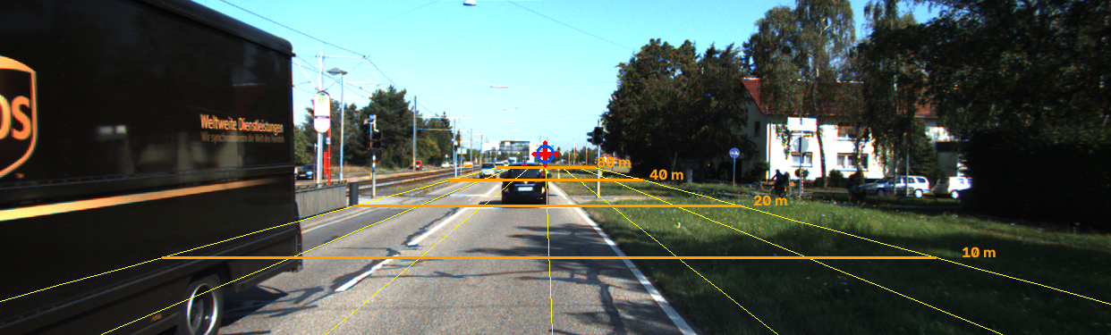
Project a grid of road-plane points onto the image: lines running parallel to the road at several \(X\) offsets, and cross lines at several distances \(Z\). Draw them on the image and label the distances.

If your grid lies flat on the road surface and the cross lines land plausibly, your projection is right. This is the check for the whole lab — if the grid floats above the road or skews off to one side, fix it before continuing.

Verify against the image: does your 10 m line fall about where you would expect a car two lengths ahead to sit?

Part 3: Vanishing points

Task 7: predict it

Lines in the world that are parallel to each other but not parallel to the image plane converge to a vanishing point.

Take your grid lines running along the road direction and let \(Z \to \infty\). Show, algebraically, where the projection ends up. Then evaluate it for this camera.

You should find that the vanishing point of the road direction lands on a familiar pair of numbers. Say what it is, and explain why it must be so, given where the optical axis is pointing in these scenes.

Task 8: measure it

Now do it the other way round — from the image alone, without the calibration.

Pick two or more points along each of two road-parallel lines (lane markings are ideal), fit a line through each, and intersect them. Report the intersection.

Compare against your predicted vanishing point from Task 7. Report the discrepancy in pixels, and account for it: some is your clicking, and some is real — the road is not perfectly straight and the car is not perfectly aligned with it.

Task 9: why this is useful

The vanishing point is a free constraint on where a road boundary can be. Say in a sentence or two how you could use it to reject a candidate road-boundary line. You will want this in Lab 6.

Part 4: Back-projection — measuring the world

Projection throws away depth: every point along a ray maps to the same pixel. But if you know the point lies on a known plane, you can recover it.

Task 10: the ray

Given a pixel \((u,v)\), the corresponding ray direction in camera coordinates is \[ \mathbf{d} \propto K^{-1}\left[\begin{array}{c}u\\v\\1\end{array}\right]. \]

Implement this. Verify it by round-tripping: project a known 3D point, take the resulting pixel, back-project the ray, and confirm the original point lies on it.

Task 11: intersect with the road

Points on the road satisfy \(Y = h\). Find the scalar \(\lambda\) such that \(\lambda\mathbf{d}\) has \(Y = h\), and hence recover the 3D point.

Write

def pixel_to_road(P, h, u, v):    # returns (X, Z) in metres, or None
    ...

Return None for pixels at or above the horizon — their rays never meet the road plane, or meet it behind the camera. Handle that case explicitly rather than returning a nonsense number.

Task 12: measure something

Use your function to:

1. Click a point on the road at the base of a vehicle ahead, and report how far away it is in metres.
2. Click the two sides of a lane at some distance and report the lane width. Standard lane widths are around 3 to 3.7 m — how close do you get?
3. Repeat the lane-width measurement at 10 m and at 40 m. Report both. Which is more accurate, and why?

Task 12.3 is the important one. Explain what happens to your measurement precision as distance grows, in terms of how many metres of road one pixel covers.

Task 13 (optional): bird’s-eye view

Apply pixel_to_road to every pixel below the horizon and re-plot the scene from directly above, with metric axes.

Straight road boundaries become straight lines in this view, and stay parallel instead of converging. That property makes fitting them much easier, which is worth remembering when you hit Lab 6.

Deliverables

Your notebook must contain the following.

• A table of \(f_x\), \(f_y\), \((c_x,c_y)\), skew, horizontal FOV and camera height, with units, plus your three sanity checks and a comment on where the principal point sits relative to the image centre.
• A table of projected pixel coordinates for \(Z = 5, 10, 20, 50\) m.
• The road-grid figure (Task 6). This is the gate for the whole lab — if the grid does not lie on the road, everything after it is suspect.
• The vanishing point derived algebraically and evaluated numerically, plus the value you measured from the image and the discrepancy in pixels, accounted for.
• pixel_to_road, with the above-horizon case returning None.
• Lane-width measurements at 10 m and at 40 m, and your explanation of why they differ in accuracy.

Submission

Via Canvas. Please submit a single executed Jupyter notebook — one that has been run top to bottom, so that every figure and number listed above is visible in the submitted file. Code that has not been executed cannot be marked.

Parting thoughts

• Do the linear algebra with numpy directly. There is no need for OpenCV’s calibration functions here, and using them hides the thing you are meant to be learning.
• Homogeneous coordinates are only awkward until you have written the divide once. Make project do the division internally so you never forget it.
• Watch the sign of \(Y\). Camera \(+Y\) points down, so the road is at positive \(h\), not negative. Getting this backwards projects your grid into the sky, which at least fails obviously.
• The camera height and the road plane are the only world measurements in this entire lab. Everything else — distances, lane widths, the bird’s-eye view — comes out of one image plus that single number. That is a good illustration of how much geometry buys you before any learning is involved.