Least squares

Faisal Qureshi
Professor
Faculty of Science
Ontario Tech University
Oshawa ON Canada
http://vclab.science.ontariotechu.ca

Copyright information

© Faisal Qureshi

License

This work is licensed under a Creative Commons Attribution-NonCommercial 4.0 International License.

import numpy as np
import matplotlib.pyplot as plt
import matplotlib.cm as cm

Lesson Plan

• Model fitting: Why?
• Linear regression
• Least squares
  • 2D line fitting example
• Total least squares
• Aside: Singular Value Decomposition (SVD)

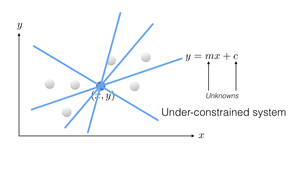
Why model fitting?

Finding objects/elements in an image

Image analysis and scene understanding

Least squares

2D line fitting example

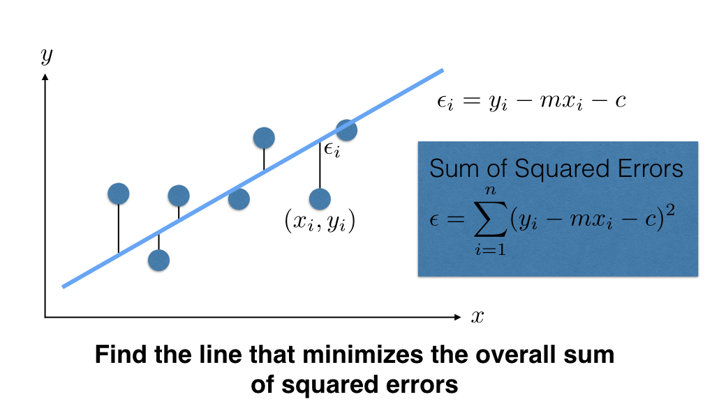
Sum of square differences is

$$ \epsilon = \sum_{i=1}^n (y_i - m x_i - c)^2 $$

We want to find values of slope $m$ and intercept $c$ so as to minimize the sum of squared differences $\epsilon$. Note that $\epsilon$ is a quadratic function (bowl shaped).

Quadratic function in 1D

$$ y = f(x) = (x + 4)^2 $$

plotting_x = np.linspace(-10,10,100)
quadratic_fn_1d = (plotting_x+4)**2

plt.figure(figsize=(5,5))
plt.title("Quadractic function in 1d")
plt.plot(plotting_x, quadratic_fn_1d)
plt.yticks([0])
plt.xticks([-4])

([<matplotlib.axis.XTick at 0x112675400>], [Text(-4, 0, '−4')])

The derivation of $f(x)$ is $$ \frac{d y}{d x} = 2(x + 4) $$

By setting $$ \frac{d y}{d x} = 0 $$ we can find the value of $x$ that minimizes function $f(x)$. In this case it is $x=-4$.

deriv_quadratic_fn_1d = 2*(plotting_x + 4)

plt.figure(figsize=(5,5))
plt.title("Quadractic function in 1d")
plt.plot(plotting_x, quadratic_fn_1d, label='$f(x)$')
plt.plot(plotting_x, deriv_quadratic_fn_1d, label="$f'(x)$")
plt.legend()
plt.yticks([0])
plt.xticks([-4])

([<matplotlib.axis.XTick at 0x1126f2210>], [Text(-4, 0, '−4')])

Quadratic function in 2D

plotting_x = np.linspace(-2,2,11)
plotting_y = np.linspace(-2,2,11)

xx, yy = np.meshgrid(plotting_x, plotting_y)

quadratic_fn_2d = xx**2 + yy**2

from mpl_toolkits.mplot3d import Axes3D
fig = plt.figure(figsize=(14,6))
ax = fig.add_subplot(121, projection='3d')
ax.plot_surface(xx, yy, quadratic_fn_2d)
plt.xlabel('x')
plt.ylabel('y')
plt.xticks([])
plt.yticks([])
plt.subplot(122)
plt.imshow(quadratic_fn_2d, extent=[-2,2,-2,2])
plt.xlabel('x')
plt.ylabel('y')
plt.xticks([0.0])
plt.yticks([0.0])
plt.suptitle('2D quadratic function');

Solving for $m$ and $c$.

$$ \DeclareMathOperator*{\argmin}{arg\,min} m^*,c^* = \argmin_{m,c} \sum_{i=1}^n \left(y_i - m x_i - c \right)^2 $$

We can achieve this by setting $$ \frac{\partial \epsilon}{\partial m} = 0 $$ and $$ \frac{\partial \epsilon}{\partial c} = 0. $$

From calculus, we know that $$ \frac{\partial \epsilon}{\partial m} = - \sum_{i=1}^n 2 x_i \left(y_i - m x_i - c \right) $$ and $$ \frac{\partial \epsilon}{\partial c} = - \sum_{i=1}^n 2 \left(y_i - m x_i - c \right). $$

Setting these to 0, we get $$ \sum_{i=1}^n 2 x_i \left(y_i - m x_i - c \right) = 0 $$ and $$ \sum_{i=1}^n 2 \left(y_i - m x_i - c \right) = 0. $$

Let $$\langle y \rangle = \frac{1}{n} \sum_{i=1}^n y_i$$ and $$\langle x \rangle = \frac{1}{n} \sum_{i=1}^n x_i.$$

We can then re-write equation 2 above as $$ c = \langle y \rangle - m \langle x \rangle. $$

Re-write equation 1 above. $$ \begin{align} & \sum_{i=1}^n x_i y_i - m \sum_{i=1}^n x_i^2 - c \sum_{i=1}^n x_i = 0 \\ \Rightarrow & \frac{1}{n} \sum_{i=1}^n x_i y_i - \frac{m}{n} \sum_{i=1}^n x_i^2 - \frac{c}{n} \sum_{i=1}^n x_i = 0 \\ \Rightarrow & \langle x y \rangle - m \langle x^2 \rangle = c \langle x \rangle \end{align} $$ where $$ \langle x y \rangle = \frac{1}{n} \sum_{i=1}^n x_i y_i $$ and $$ \langle x^2 \rangle = \frac{1}{n} \sum_{i=1}^n x_i^2. $$

Substitute the value of $c$ $$ \begin{align} & \langle x y \rangle - m \langle x^2 \rangle = \langle x \rangle \langle y \rangle - m \langle x \rangle^2 \\ \Rightarrow & m \left( \langle x \rangle^2 - \langle x^2 \rangle \right) = \langle x \rangle \langle y \rangle - \langle x y \rangle \\ \Rightarrow & m = \frac{\langle x \rangle \langle y \rangle - \langle x y \rangle}{\langle x \rangle^2 - \langle x^2 \rangle} \end{align} $$

Use this value of $m$ to solve for $c$.

2D line fitting example 1

# Generate some data
np.random.seed(0)

m_true = .75
c_true = 1

x = np.hstack([np.linspace(3, 5, 5), np.linspace(7, 8, 5)])
y = m_true * x + c_true + np.random.rand(len(x))
data = np.vstack([x, y]).T
n = data.shape[0]

plt.figure(figsize=(7,7))
plt.scatter(data[:,0], data[:,1], c='red', alpha=0.9)
plt.xlim([0,10])
plt.ylim([0,10])
plt.title('Generating some points from a line');

x = data[:,0]
y = data[:,1]

print(f'x =\n{x.reshape(n,1)}')
print(f'y =\n{y.reshape(n,1)}')

x =
[[3.  ]
 [3.5 ]
 [4.  ]
 [4.5 ]
 [5.  ]
 [7.  ]
 [7.25]
 [7.5 ]
 [7.75]
 [8.  ]]
y =
[[3.7988135 ]
 [4.34018937]
 [4.60276338]
 [4.91988318]
 [5.1736548 ]
 [6.89589411]
 [6.87508721]
 [7.516773  ]
 [7.77616276]
 [7.38344152]]

mean_x = np.mean(x)
mean_y = np.mean(y)
mean_x2 = np.mean(np.square(x))
mean_xy = np.mean(x * y)

print(f'<x> = {mean_x}')
print(f'<y> = {mean_y}')
print(f'<x2> = {mean_x2}')
print(f'<xy> = {mean_xy}')

<x> = 5.75
<y> = 5.928266283314543
<x2> = 36.4375
<xy> = 36.68301372420285

m = (mean_x * mean_y - mean_xy) / (mean_x**2 - mean_x2)
print(f'm = {m}')

m = 0.7690318800427336

c = mean_y - mean_x * m
print(f'c = {c}')

c = 1.506332973068825

x_plotting = np.linspace(0,10,100)
y_plotting = m * x_plotting + c

plt.figure(figsize=(7,7))
plt.scatter(data[:,0], data[:,1], c='red', alpha=0.9)
plt.plot(x_plotting, y_plotting, 'b-')
plt.xlim([0,10])
plt.ylim([0,10])
plt.title('Line fitted to data using least squares.')

Text(0.5, 1.0, 'Line fitted to data using least squares.')

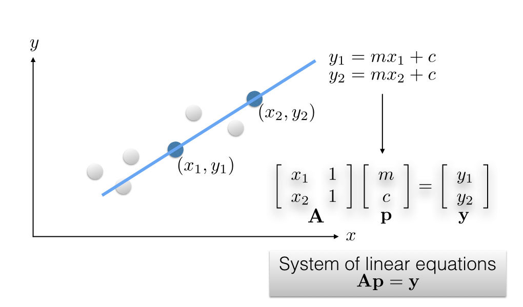
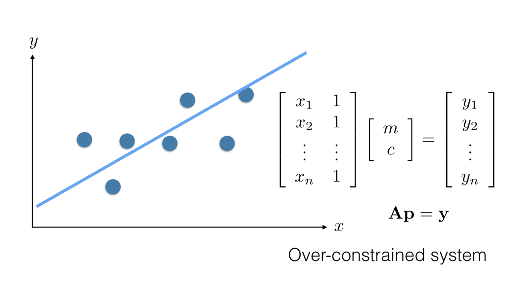
2D line fitting - vector notation

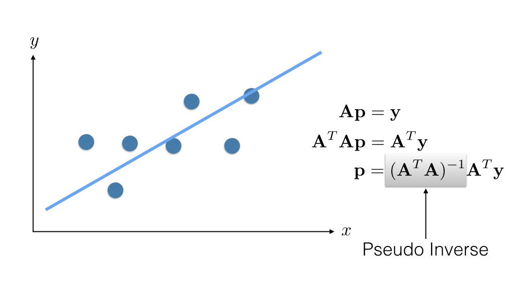
$$ \begin{align} \epsilon &= \sum_{i=1}^n (y_i - m x_i - c)^2 \\ &= \| \left[ \begin{array}{c} y_1 \\ y_2 \\ \vdots \\ y_n \end{array} \right] - \left[ \begin{array}{cc} x_1 & 1\\ x_2 & 1\\ \vdots & \vdots \\ x_n & 1 \end{array} \right] \left[ \begin{array}{c} m\\ c \end{array} \right] \|^2 \\ &= \| \mathbf{y} - \mathbf{A} \mathbf{p} \|^2 \\ &= \mathbf{y}^T\mathbf{y} - 2 ( \mathbf{A} \mathbf{p} )^T \mathbf{y} + (\mathbf{A} \mathbf{p})^T \mathbf{A} \mathbf{p} \end{align} $$

We know that $$ \frac{\partial \epsilon}{\partial \mathbf{p}} = -2 \mathbf{A}^T \mathbf{y} + 2 \mathbf{A}^T \mathbf{A} \mathbf{p} $$

Setting $$ \frac{\partial \epsilon}{\partial \mathbf{p}}=0. $$ we get $$ \begin{align} & -2 \mathbf{A}^T \mathbf{y} + 2 \mathbf{A}^T \mathbf{A} \mathbf{p} = 0 \\ \Rightarrow & \mathbf{A}^T\mathbf{A} \mathbf{p} = \mathbf{A}^T \mathbf{y} \\ \Rightarrow & \mathbf{p} = (\mathbf{A}^T\mathbf{A})^{-1} \mathbf{A}^T \mathbf{y} \end{align} $$

$(\mathbf{A}^T\mathbf{A})^{-1}$ is called the psuedo inverse $\mathbf{A}$.

2D line fitting - intuition - linear algebra

2D line fitting example 2

# Generate some data
np.random.seed(0)

m_true = .75
c_true = 1

x = np.hstack([np.linspace(3, 5, 5), np.linspace(7, 8, 5)])
y = m_true * x + c_true + np.random.rand(len(x))

#x = np.linspace(1,9,10)
#y = np.ones(10)+5

#y = np.linspace(1,9,10)
#x = np.ones(10)+5

data = np.vstack([x, y]).T
n = data.shape[0]

plt.figure(figsize=(7,7))
plt.scatter(data[:,0], data[:,1], c='red', alpha=0.9)
plt.xlim([0,10])
plt.ylim([0,10])
plt.title('Generating some points from a line')

Text(0.5, 1.0, 'Generating some points from a line')

print(f'data =\n{data}')
n = data.shape[0]
print(f'Number of data items = {n}')

data =
[[3.         3.7988135 ]
 [3.5        4.34018937]
 [4.         4.60276338]
 [4.5        4.91988318]
 [5.         5.1736548 ]
 [7.         6.89589411]
 [7.25       6.87508721]
 [7.5        7.516773  ]
 [7.75       7.77616276]
 [8.         7.38344152]]
Number of data items = 10

A = np.ones([n, 2])
A[:,0] = data[:,0]
print(f'A =\n{A}')

A =
[[3.   1.  ]
 [3.5  1.  ]
 [4.   1.  ]
 [4.5  1.  ]
 [5.   1.  ]
 [7.   1.  ]
 [7.25 1.  ]
 [7.5  1.  ]
 [7.75 1.  ]
 [8.   1.  ]]

AtA = np.dot(A.T,A)
print(f'AtA =\n {AtA}')

AtA =
 [[364.375  57.5  ]
 [ 57.5    10.   ]]

AtY = np.dot(A.T, data[:,1].reshape(n,1))
print(f'AtY = \n{AtY}')

AtY = 
[[366.83013724]
 [ 59.28266283]]

# m = slope
# c = intercept
m_and_c = np.dot(np.linalg.inv(AtA), AtY)

m = m_and_c[0]
c = m_and_c[1]

print(f'm = {m}')
print(f'c = {c}')

m = [0.76903188]
c = [1.50633297]

x_plotting = np.linspace(0,10,100)
y_plotting = m * x_plotting + c

plt.figure(figsize=(7,7))
plt.scatter(data[:,0], data[:,1], c='red', alpha=0.9)
plt.plot(x_plotting, y_plotting, 'b-')
plt.xlim([0,10])
plt.ylim([0,10])
plt.title('Line fitted to data using least squares.');

Total least squares

2D line fitting example

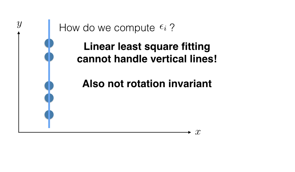
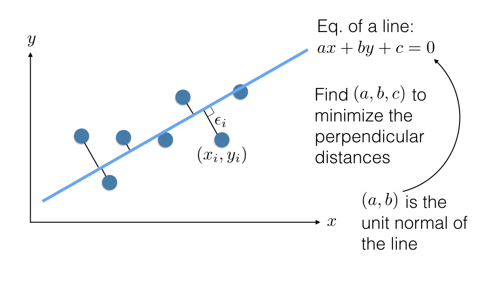
Solving for $a$, $b$, and $c$

Minimize $$ \epsilon = \sum_{i=1}^n (a x_i + b y_i + c)^2\mathrm{\ s.t.\ } (a,b)^T(a,b) = 1 $$

From calculus $$ \frac{\partial \epsilon}{\partial c} = 2 \sum_{i=1}^n (a x_i + b y_i + c). $$ Setting $$ \frac{\partial \epsilon}{\partial c} = 0, $$ we get $$ \begin{align} & \sum_{i=1}^n (a x_i + b y_i + c) = 0 \\ \Rightarrow & a \sum_{i=1}^n x_i + b \sum_{i=1}^n y_i + n c = 0 \\ \Rightarrow & c = - \frac{a \sum_{i=1}^n x_i}{n} - \frac{b \sum_{i=1}^n y_i}{n}\\ \Rightarrow & c = - a \langle x \rangle - b \langle y \rangle \end{align} $$

Substituting $c$ back in $\epsilon$ $$ \begin{align} \epsilon &= \sum_{i=1}^n \left[a x_i + b y_i + \left(- a \langle x \rangle - b \langle y \rangle\right)\right]^2 \\ &= \sum_{i=1}^n \left[ a \left( x_i - \langle x \rangle \right) + b \left( y_i - \langle y \rangle \right) \right]^2 \\ &= \| \left[ \begin{array}{cc} x_1 - \langle x \rangle & y_1 - \langle y \rangle \\ x_2 - \langle x \rangle & y_2 - \langle y \rangle \\ \vdots & \vdots \\ x_n - \langle x \rangle & y_n - \langle y \rangle \\ \end{array} \right] \left[ \begin{array}{c} a \\ b \end{array} \right] \|^2 \\ &= \| \mathbf{A} \mathbf{p} \|^2 \end{align} $$

Note that this is not the same $\mathbf{A}$ as the one that we constructed for linear least squares.

We can thus re-write our problem as $$ \DeclareMathOperator*{\argmin}{arg\,min} \mathbf{p}^* = \argmin_\mathbf{p} \| \mathbf{A} \mathbf{p} \|^2 \mathrm{\ s.t.\ }\mathbf{p}^T\mathbf{p} = 1. $$

Solution is the eigenvector corresponding to the smallest eigenvalues of $\mathbf{A}^T\mathbf{A}$.

2D line fitting example 3

# Generate some data
np.random.seed(0)

m_true = .75
c_true = 1

# x = np.hstack([np.linspace(3, 5, 5), np.linspace(7, 8, 5)])
# y = m_true * x + c_true + np.random.rand(len(x))\

#x = np.linspace(1,9,10)
#y = np.ones(10)+5

y = np.linspace(1,9,10)
x = np.ones(10)+1

data = np.vstack([x, y]).T
n = data.shape[0]

plt.figure(figsize=(7,7))
plt.scatter(data[:,0], data[:,1], c='red', alpha=0.9)
plt.xlim([0,10])
plt.ylim([0,10])
plt.title('Generating some points from a line')

Text(0.5, 1.0, 'Generating some points from a line')

print(np.vstack((x,y)))

[[2.         2.         2.         2.         2.         2.
  2.         2.         2.         2.        ]
 [1.         1.88888889 2.77777778 3.66666667 4.55555556 5.44444444
  6.33333333 7.22222222 8.11111111 9.        ]]

print(f'x =\n {data[:,0].reshape(n,1)}')

x =
 [[2.]
 [2.]
 [2.]
 [2.]
 [2.]
 [2.]
 [2.]
 [2.]
 [2.]
 [2.]]

mean_x = np.mean(data[:,0])
print(f'mean_x = {mean_x}')

mean_x = 2.0

print(f'y =\n {data[:,1].reshape(n,1)}')

y =
 [[1.        ]
 [1.88888889]
 [2.77777778]
 [3.66666667]
 [4.55555556]
 [5.44444444]
 [6.33333333]
 [7.22222222]
 [8.11111111]
 [9.        ]]

mean_y = np.mean(data[:,1])
print(f'mean_x = {mean_y}')

mean_x = 5.0

A = np.hstack([(x-mean_x).reshape(n,1), (y-mean_y).reshape(n,1)])
print(f'A =\n{A}')

A =
[[ 0.         -4.        ]
 [ 0.         -3.11111111]
 [ 0.         -2.22222222]
 [ 0.         -1.33333333]
 [ 0.         -0.44444444]
 [ 0.          0.44444444]
 [ 0.          1.33333333]
 [ 0.          2.22222222]
 [ 0.          3.11111111]
 [ 0.          4.        ]]

AtA = np.dot(A.T, A)
print(f'AtA =\n{AtA}')

AtA =
[[ 0.          0.        ]
 [ 0.         65.18518519]]

e, v = np.linalg.eig(AtA)
print(f'eigenvalues = \n{e}')
print(f'eigenvectors = \n{v}')

eigenvalues = 
[ 0.         65.18518519]
eigenvectors = 
[[1. 0.]
 [0. 1.]]

smallest_eigen_value_index = np.argmin(e)
print(f'Index for smallest eigenvalue = {smallest_eigen_value_index}')

Index for smallest eigenvalue = 0

p = v[:, smallest_eigen_value_index]
print(f'Eigenvector corresponding to the smallest eigenvector =\n{p}')

Eigenvector corresponding to the smallest eigenvector =
[1. 0.]

a = p[0]
b = p[1]
c = - a * mean_x - b * mean_y

print(f'a = {a}, b={b}, and c={c}')

print(f'Equation of the line is: x={-c/a}')

a = 1.0, b=0.0, and c=-2.0
Equation of the line is: x=2.0

plotting_x = np.linspace(0, 10, 100)
plotting_y = np.linspace(0, 10, 100)
xx, yy = np.meshgrid(plotting_x, plotting_y)
z = a * xx + b * yy + c

fig = plt.figure(figsize=(7,7))
plt.imshow(z, origin='lower', extent=(0,10,0,10))
plt.colorbar()
plt.contour(xx, yy, z, [0])
plt.scatter(data[:,0], data[:,1], c='red', alpha=0.9)
plt.xlim([0,10])
plt.ylim([0,10])
plt.title('Line fitted using total least squares')

Text(0.5, 1.0, 'Line fitted using total least squares')

A = np.vstack((x,y,np.ones(len(x)))).T
print(A)

AtA = np.dot(A.T,A)
print(AtA)

e, v = np.linalg.eig(AtA)
print(f'eigenvalues = \n{e}')
print(f'eigenvectors = \n{v}')

smallest_eigen_value_index = np.argmin(e)
print(f'Index for smallest eigenvalue = {smallest_eigen_value_index}')

p = v[:, smallest_eigen_value_index]
print(f'Eigenvector corresponding to the smallest eigenvector =\n{p}')

a, b, c = p[0], p[1], p[2]
print(f'a = {a}, b={b}, and c={c}')

plotting_x = np.linspace(0, 10, 100)
plotting_y = np.linspace(0, 10, 100)
xx, yy = np.meshgrid(plotting_x, plotting_y)
z = a * xx + b * yy + c

fig = plt.figure(figsize=(7,7))
plt.imshow(z, origin='lower', extent=(0,10,0,10))
plt.colorbar()
plt.contour(xx, yy, z, [0])
plt.scatter(data[:,0], data[:,1], c='red', alpha=0.9)
plt.xlim([0,10])
plt.ylim([0,10])
plt.title('Line fitted using total least squares')

print(f'Equation of the line is: x={-c/a}')

[[2.         1.         1.        ]
 [2.         1.88888889 1.        ]
 [2.         2.77777778 1.        ]
 [2.         3.66666667 1.        ]
 [2.         4.55555556 1.        ]
 [2.         5.44444444 1.        ]
 [2.         6.33333333 1.        ]
 [2.         7.22222222 1.        ]
 [2.         8.11111111 1.        ]
 [2.         9.         1.        ]]
[[ 40.         100.          20.        ]
 [100.         315.18518519  50.        ]
 [ 20.          50.          10.        ]]
eigenvalues = 
[ 3.56030753e+02  9.15443183e+00 -3.00994406e-15]
eigenvectors = 
[[-3.06923496e-01 -8.40117829e-01 -4.47213595e-01]
 [-9.39280288e-01  3.43150901e-01  3.42758055e-16]
 [-1.53461748e-01 -4.20058915e-01  8.94427191e-01]]
Index for smallest eigenvalue = 2
Eigenvector corresponding to the smallest eigenvector =
[-4.47213595e-01  3.42758055e-16  8.94427191e-01]
a = -0.44721359549995876, b=3.4275805455575054e-16, and c=0.8944271909999155
Equation of the line is: x=1.9999999999999956

Aside: Singular Value Decomposition (SVD)

SVD of a matrix $\mathbf{A} \in \mathbb{R}^{m \times n}$ is defined as $$ \mathbf{A} = \mathbf{U} \mathbf{D} \mathbf{V}^T $$ such that $\mathbf{U}$ is an $m \times n$ matrix with orthognal columns, $\mathbf{D}$ is an $n \times n$ diagonal matrix containing singular values, and $\mathbf{V}$ is an $n \times n$ orthognal matrix.

The column of $\mathbf{V}$ corresponding to the smallest singular value in $\mathbf{D}$ is the smallest eigenvector of $\mathbf{A}^T \mathbf{A}$.