Texture analysis

Faisal Qureshi
Professor
Faculty of Science
Ontario Tech University
Oshawa ON Canada
http://vclab.science.ontariotechu.ca

Copyright information

© Faisal Qureshi

License

This work is licensed under a Creative Commons Attribution-NonCommercial 4.0 International License.

Lesson Plan

• Texture analysis
• Filter banks
  • Leung-Malik Filter (LM) Bank
    • LM filter construction
  • Schmid Filter Bank
  • Maximum Response Filter Bank

import numpy as np
import cv2 as cv
import matplotlib.pyplot as plt
import scipy as sp
from scipy import signal
from scipy import io
from scipy.spatial import distance

The Leung-Malik (LM) Filter Bank

The LM set is a multi-scale, multi-orientation filter bank with 48 filters. It consists of first and second derivatives of Gaussians at 6 orientations and 3 scales making a total of 36; 8 Laplacian of Gaussian (LOG) filters; and 4 Gaussians.

LM Small (LMS) filters occur at scales $\sigma = \{1, \sqrt{2}, 2, 2 \sqrt{2} \}$. The first and second derivates occur at the first three scales with an elongation factor of 3 (i.e., $\sigma_x = \sigma$ and $\sigma_y = 3 \sigma$). The Gaussians occuer at four basic scales. The 8 LOG occur at $\sigma$ and $3 \sigma$.

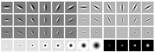
Figure from https://www.robots.ox.ac.uk/~vgg/research/texclass/filters.html.

LM Large (LML) filters occur at scales $\sigma = \{ \sqrt{2},2,2\sqrt{2},4 \}$.

LM filter construction

F = sp.io.loadmat('data/lm.mat')
#print(F)
print(F['LM'].shape)

(49, 49, 48)

filter_bank = F['LM']
nr = 4
nc = 48//nr
plt.figure(figsize=(14,5))
plt.suptitle('LM filters.  ')
for i in range(48):
    plt.subplot(nr, nc, i+1)
    fig = plt.imshow(filter_bank[:,:,i], cmap='gray')
    fig.axes.get_xaxis().set_visible(False)
    fig.axes.get_yaxis().set_visible(False)
plt.show()    

feature_vectors = np.empty((4,48))  # we will use this to store feature vectors.

filenames = [
    'data/textures/banded_0023.jpg',
    'data/textures/interlaced_0201.jpg',
    'data/textures/knitted_0204.jpg',
    'data/textures/lined_0177.jpg', 
    'data/textures/sprinkled_0144.jpg', 
    'data/textures/studded_0217.jpg', 
    'data/textures/woven_0131.jpg', 
    'data/textures/zigzagged_0133.jpg',
    'data/textures/matted_0166.jpg'
]
f_idx = 1

im = cv.imread(filenames[f_idx], 0)
print(im.shape)

plt.figure(figsize=(5,5))
plt.imshow(im, cmap='gray');

(300, 300)

w, h = im.shape
_, _, num_filters = filter_bank.shape
responses = np.empty([w, h, num_filters])
print(responses.shape)

(300, 300, 48)

for i in range(num_filters):
    responses[:,:,i] = sp.signal.convolve(im, filter_bank[:,:,i], mode='same')

plt.figure(figsize=(14,5))
plt.suptitle('LM filter responses')
for i in range(48):
    plt.subplot(nr, nc, i+1)
    fig = plt.imshow(responses[:,:,i], cmap='gray')
    fig.axes.get_xaxis().set_visible(False)
    fig.axes.get_yaxis().set_visible(False)
plt.show() 

# fv = np.empty(48)
# for i in range(48):
#     fv[i] = np.mean(responses[:,:,i])

fv = np.mean(responses,(0,1)).flatten()
fv2 = np.std(responses,(0,1)).flatten()
ffv = np.hstack((fv, fv2))

x = np.linspace(0, 95, 96, endpoint=True)

plt.figure(figsize=(10,5))
plt.bar(x, ffv, color='red')
plt.title(f'{filenames[f_idx]}')
plt.ylim(-5,5);

def make_responses(filter_bank, filenames):
    _, _, num_filters = filter_bank.shape        
    num_files = len(filenames)

    feature_vectors = np.empty((num_files, num_filters))
    
    for i in range(num_files):
        filename = filenames[i]
        print(f'Processing {filename}')

        im = cv.imread(filename, 0)
        for j in range(num_filters):
            feature_vectors[i,j] = np.mean(sp.signal.convolve(im, filter_bank[:,:,j], mode='same'))
    
    return feature_vectors

fv = make_responses(filter_bank, filenames)

Processing data/textures/banded_0023.jpg
Processing data/textures/interlaced_0201.jpg
Processing data/textures/knitted_0204.jpg
Processing data/textures/lined_0177.jpg

Processing data/textures/sprinkled_0144.jpg
Processing data/textures/studded_0217.jpg
Processing data/textures/woven_0131.jpg
Processing data/textures/zigzagged_0133.jpg

Processing data/textures/matted_0166.jpg

x = np.linspace(0, 47, 48, endpoint=True)

plt.figure(figsize=(10,5))
plt.bar(x, fv[0,:], color='red', alpha=0.3)
plt.bar(x, fv[1,:], color='blue', alpha=0.3)
plt.bar(x, fv[2,:], color='green', alpha=0.3)
plt.bar(x, fv[3,:], color='cyan', alpha=0.3)
plt.title(f'{filenames[f_idx]}')
plt.ylim(-5,5);

D = distance.squareform(distance.pdist(fv, 'euclidean'))
print(D)

[[ 0.          1.17007043  1.96303145  1.95019134  6.50901116  4.56143119
   1.72228842  2.43435123  3.34896037]
 [ 1.17007043  0.          3.03348622  1.10738299  5.46341285  5.62859271
   0.67168458  1.42188238  2.27504938]
 [ 1.96303145  3.03348622  0.          3.44827149  8.33153977  2.92493385
   3.61802594  4.15907937  5.21627558]
 [ 1.95019134  1.10738299  3.44827149  0.          5.30653314  6.06491459
   1.25390674  1.28007894  2.28311881]
 [ 6.50901116  5.46341285  8.33153977  5.30653314  0.         11.0668718
   4.83289756  4.24947566  3.19409886]
 [ 4.56143119  5.62859271  2.92493385  6.06491459 11.0668718   0.
   6.24536833  6.91161908  7.88883183]
 [ 1.72228842  0.67168458  3.61802594  1.25390674  4.83289756  6.24536833
   0.          0.94956252  1.64941744]
 [ 2.43435123  1.42188238  4.15907937  1.28007894  4.24947566  6.91161908
   0.94956252  0.          1.2388296 ]
 [ 3.34896037  2.27504938  5.21627558  2.28311881  3.19409886  7.88883183
   1.64941744  1.2388296   0.        ]]

The Schmid (S) Filters

The S set consists of 13 rotationally invariant filters of the form

$$ F(r, \sigma, \tau) = F_0 (\sigma, r) + \cos \left( \frac{\pi \tau r}{\sigma} \right) e ^ { - \frac{r^2}{2 \sigma^2} } $$

Schmid Filter Bank equation where $F_{0}$ is added to obtain a zero DC component with the $(\sigma, \tau)$ pair taking values $(2,1)$, $(4,1)$, $(4,2)$, $(6,1)$, $(6,2)$, $(6,3)$, $(8,1)$, $(8,2)$, $(8,3)$, $(10,1)$, $(10,2)$, $(10,3)$ and $(10,4)$. The filters are shown below.

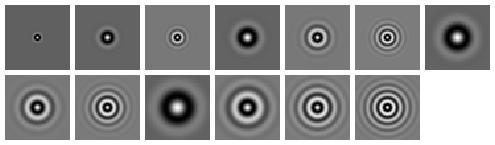
Figure from https://www.robots.ox.ac.uk/~vgg/research/texclass/filters.html.

All the filters have rotational symmetry.

F = sp.io.loadmat('data/s.mat')
print(F['S'].shape)

filter_bank = F['S']
nr = 2
nc = int(np.ceil(13/nr))
plt.figure(figsize=(14,5))
plt.suptitle('S filters.  ')
for i in range(13):
    plt.subplot(nr, nc, i+1)
    fig = plt.imshow(filter_bank[:,:,i], cmap='gray')
    fig.axes.get_xaxis().set_visible(False)
    fig.axes.get_yaxis().set_visible(False)
plt.show()    

(49, 49, 13)

fv = make_responses(filter_bank, filenames)

Processing data/textures/banded_0023.jpg
Processing data/textures/interlaced_0201.jpg
Processing data/textures/knitted_0204.jpg
Processing data/textures/lined_0177.jpg
Processing data/textures/sprinkled_0144.jpg
Processing data/textures/studded_0217.jpg
Processing data/textures/woven_0131.jpg
Processing data/textures/zigzagged_0133.jpg
Processing data/textures/matted_0166.jpg

x = np.linspace(0, 12, 13, endpoint=True)

plt.figure(figsize=(10,5))
plt.bar(x, fv[0,:], color='red', alpha=0.3)
plt.bar(x, fv[1,:], color='blue', alpha=0.3)
plt.bar(x, fv[2,:], color='green', alpha=0.3)
plt.bar(x, fv[3,:], color='cyan', alpha=0.3)
plt.title(f'{filenames[f_idx]}')
plt.ylim(-5,5);

The Maximum Response (MR) Filter Banks

Each of the reduced MR sets is derived from a common Root Filter Set (RFS) which consists of 38 filters and is very similar to LM. The filters used in the RFS bank are a Gaussian and a Laplacian of Gaussian both with $\sigma=10$ pixels (these filters have rotational symmetry), an edge filter at 3 scales (scale values) = $\{(1,3), (2,6), (4,12)\}$ and a bar filter at the same 3 scales. The latter two filters are oriented and, as in LM, occur at 6 orientations at each scale. The filter bank is shown below.

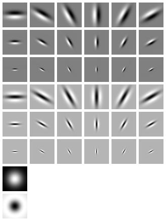
Figure from https://www.robots.ox.ac.uk/~vgg/research/texclass/filters.html.

F = sp.io.loadmat('data/rfs.mat')
print(F['RFS'].shape)

filter_bank = F['RFS']
nr = 3

nc = np.ceil(38/nr)
plt.figure(figsize=(14,4))
plt.suptitle('S filters.  ')
for i in range(38):
    plt.subplot(int(nr), int(nc), i+1)
    fig = plt.imshow(filter_bank[:,:,i], cmap='gray')
    fig.axes.get_xaxis().set_visible(False)
    fig.axes.get_yaxis().set_visible(False)
plt.show()    

(49, 49, 38)

fv = make_responses(filter_bank, filenames)

Processing data/textures/banded_0023.jpg

Processing data/textures/interlaced_0201.jpg
Processing data/textures/knitted_0204.jpg
Processing data/textures/lined_0177.jpg
Processing data/textures/sprinkled_0144.jpg

Processing data/textures/studded_0217.jpg

Processing data/textures/woven_0131.jpg
Processing data/textures/zigzagged_0133.jpg
Processing data/textures/matted_0166.jpg

x = np.linspace(0, 37, 38, endpoint=True)

plt.figure(figsize=(10,5))
plt.bar(x, fv[0,:], color='red', alpha=0.3)
plt.bar(x, fv[1,:], color='blue', alpha=0.3)
plt.bar(x, fv[2,:], color='green', alpha=0.3)
plt.bar(x, fv[3,:], color='cyan', alpha=0.3)
plt.title(f'{filenames[f_idx]}')
plt.ylim(-5,5);