Bilateral filtering
Faisal Qureshi
Professor
Faculty of Science
Ontario Tech University
Oshawa ON Canada
http://vclab.science.ontariotechu.ca
Copyright information
© Faisal Qureshi
License

This work is licensed under a Creative Commons Attribution-NonCommercial 4.0 International License.
Lesson Plan
- Bilateral filtering
import numpy as np
import matplotlib.pyplot as plt
%matplotlib inline

np.random.seed(2)
Gaussian kernel in 1D - Review
A Gaussian kernel is a kernel with the shape of a Gaussian (Normal distribution) curve. Here is a standard Gaussian, with a mean of $0$ and a $\sigma$ of 1.
x_gaussian = np.arange(-5, 5, 0.1)
sigma = 1
y_gaussian = 1. / np.sqrt(2 * np.pi) * np.exp(-x_gaussian**2 / (2. * sigma**2))
plt.figure(figsize=(5,5))
plt.plot(x_gaussian, y_gaussian, c='r');

Full Width at Half Maximum Measure (FWHM)
When the Gaussian is used for smoothing, it is common to describe the width of the Gaussian in terms of the Full Width at Half Maximum (FWHM). The FWHM is the width of the kernel, at half of the maximum of the height of the Gaussian.
In the above example, the maximum value for the Gaussian is ~$0.4$. The $x$ value corresponding to half the maximum value (i.e., 0.2) is roughly $-1.17$ and $1.17$. This suggests that the FWHM is ~$2 \times 1.17$.
The following python routines capture the relationship between $\sigma$ and FWHM.
def sigma2fwhm(sigma):
    return sigma * np.sqrt(8 * np.log(2))

def fwhm2sigma(fwhm):
    return fwhm / np.sqrt(8 * np.log(2))
sigma = 1
fwhm = sigma2fwhm(sigma)
print(f'fwhm at sigma = {sigma} is {fwhm}')
fwhm at sigma = 1 is 2.3548200450309493
fwhm = 2.35
sigma = fwhm2sigma(2.35)
print(f'sigma at fwhm = {fwhm} is {sigma}')
sigma at fwhm = 2.35 is 0.9979531153384225
def min(a, b):
    if a < b:
        return a
    return b

def max(a, b):
    if a < b:
        return b
    return a
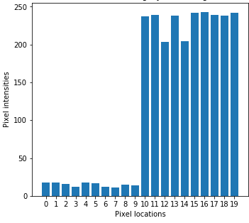
Gaussian smoothing in 1D
Lets first study the effect of Gaussian smoothing in 1D and its effect on edges.
import numpy as np
import matplotlib.pyplot as plt
np.random.seed(2)
N = 2*10 # The trick to ensure N is always even
x = np.arange(N)
x_max = np.max(x)
y_first = np.random.randint(low=10, high=20, size=N//2)
y_second = np.random.randint(low=200, high=250, size=N//2)
y = np.hstack([y_first, y_second])

plt.figure(figsize=(5,5))
plt.title('One dimensional grayscale image')
plt.ylabel('Pixel intensities')
plt.xlabel('Pixel $x$ locations')
plt.ylim(0, 255)
plt.xticks(x)
plt.bar(x, y);

Computing Smoothed Values
In order to smooth data using a Gaussian kernel, we need to slide the kernel over the signal and recompute corresponding values. Consider the signal above. Say we want to recompute the value at pixel location = 5. We will need to place a Gaussian at this location to compute the new value at location 5.
scale = 200 # So we can actually see it

FWHM = 8
sigma = fwhm2sigma(FWHM)
x_position = 15
kernel_at_pos = np.exp(-(x - x_position) ** 2 / (2 * sigma ** 2))
kernel_at_pos = kernel_at_pos / np.sum(kernel_at_pos)

plt.figure(figsize=(5,5))
plt.title('One dimensional grayscale image')
plt.ylabel('Pixel intensities')
plt.xlabel('Pixel $x$ locations')
plt.ylim(0, 255)
plt.xticks(x)
plt.bar(x, y)
plt.bar(x, scale*kernel_at_pos, alpha=0.5, color='r');

x_position_min = max(x_position - FWHM, 0)
x_position_max = min(x_position + FWHM, x_max)+1

print('x: {}'.format(x_position))
print('x min: {}'.format(x_position_min))
print('x max: {}'.format(x_position_max))

relevant_y = y[x_position_min:x_position_max]
relevant_k = kernel_at_pos[x_position_min:x_position_max]
smoothed_y_at_position = np.sum(relevant_y * relevant_k)

np.set_printoptions(precision=3, suppress=True)
print('Value of signal around {}:'.format(x_position), relevant_y)
print('Value of kernel around {}:'.format(x_position), relevant_k)
print('Old y at {} = {:.2f}'.format(x_position, y[x_position]))
print('New y at {} = {:.2f}'.format(x_position, smoothed_y_at_position))
x: 15
x min: 7
x max: 20
Value of signal around 15: [ 11  15  14 237 239 203 238 204 242 243 239 238 242]
Value of kernel around 15: [0.008 0.015 0.027 0.044 0.065 0.088 0.109 0.124 0.129 0.124 0.109 0.088
 0.065]
Old y at 15 = 242.00
New y at 15 = 219.30
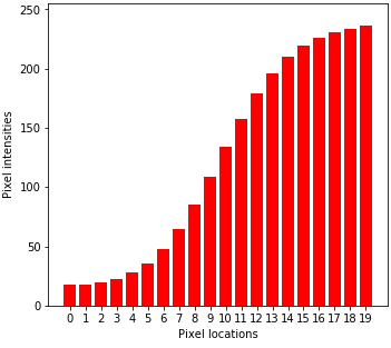
Sliding window
smoothed_y = np.zeros(y.shape)
for x_position in x:
    kernel = np.exp(-(x - x_position) ** 2 / (2 * sigma ** 2))
    kernel = kernel / np.sum(kernel)
    smoothed_y[x_position] = np.sum(y * kernel)

plt.figure(figsize=(12,5))
plt.subplot(121)
plt.title('One dimensional grayscale image')
plt.xlabel('Pixel locations')
plt.ylabel('Pixel intensities')
plt.xticks(x)
plt.ylim(0,255)
plt.bar(x, y, alpha=1)
plt.subplot(122)
plt.title('One dimensional grayscale image (Smoothed)')
plt.xlabel('Pixel locations')
plt.ylabel('Pixel intensities')
plt.xticks(x)
plt.ylim(0,255)
plt.bar(x, smoothed_y, alpha=1, color='r')
<BarContainer object of 20 artists>

Bilateral filtering in 1D
x_position = 9 # Position in array is 6 (0 based)

FWHM1 = 8 # The value falls below the half of maximum value after 2
sigma1 = fwhm2sigma(FWHM1)
kernel1_at_pos = np.exp(-(x - x_position) ** 2 / (2 * sigma1 ** 2))
kernel1_at_pos = kernel1_at_pos / np.sum(kernel1_at_pos) # Sum to 1

FWHM2 = 60 # The value falls below the half of maximum value after 2
sigma2 = fwhm2sigma(FWHM2)
kernel2_at_pos = np.zeros(kernel1_at_pos.shape)
kernel2_at_pos = np.exp(-(y[x] - y[x_position]) ** 2 / (2 * sigma2 ** 2))
kernel2_at_pos = kernel2_at_pos / np.sum(kernel2_at_pos)

scale = 200 # So we can actually see it

plt.figure(figsize=(12,5))
plt.subplot(121)
plt.title('Nearness')
plt.ylabel('Pixel intensities')
plt.xlabel('Pixel $x$ locations')
plt.ylim(0, 255)
plt.xticks(x)
plt.bar(x, y, alpha=.5)
plt.bar(x, scale*kernel1_at_pos, alpha=0.5, color='r')
plt.subplot(122)
plt.title('Same intensities')
plt.ylabel('Pixel intensities')
plt.xlabel('Pixel $x$ locations')
plt.ylim(0, 255)
plt.xticks(x)
plt.bar(x, y, alpha=.5)
plt.bar(x, scale*kernel2_at_pos, alpha=0.5, color='g');

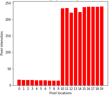
Sliding window
smoothed_y = np.zeros(y.shape)
for x_position in x:
    kernel1 = np.exp(-(x - x_position) ** 2 / (2 * sigma1 ** 2))
    kernel2 = np.exp(-(y[x] - y[x_position]) ** 2 / (2 * sigma2 ** 2))
    kernel = kernel1 * kernel2
    kernel = kernel / np.sum(kernel)
    smoothed_y[x_position] = np.sum(y * kernel)

plt.figure(figsize=(12,5))
plt.subplot(121)
plt.title('One dimensional grayscale image')
plt.xlabel('Pixel locations')
plt.ylabel('Pixel intensities')
plt.xticks(x)
plt.ylim(0,255)
plt.bar(x, y, alpha=1)
plt.subplot(122)
plt.title('One dimensional grayscale image (Smoothed)')
plt.xlabel('Pixel locations')
plt.ylabel('Pixel intensities')
plt.xticks(x)
plt.ylim(0,255)
plt.bar(x, smoothed_y, alpha=1, color='r');

Comparison
(Left to right) 1d input image, Gaussian smoothing, and bilateral filtering. Note that bilateral filtering preserves edge information.
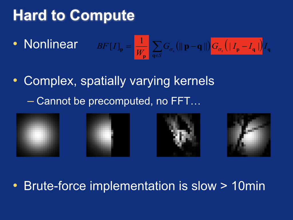
Bilateral filtering theory
The following slides on bilateral filter are taken from https://people.csail.mit.edu/sparis/bf_course.
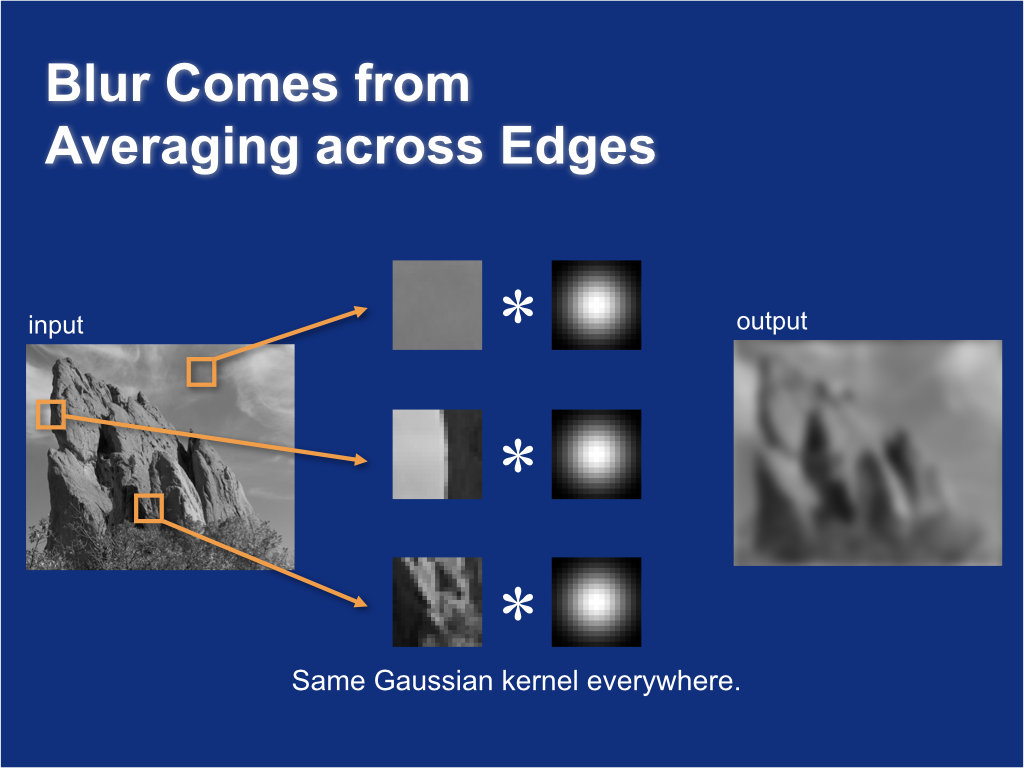
Blur comes from averaging across edges
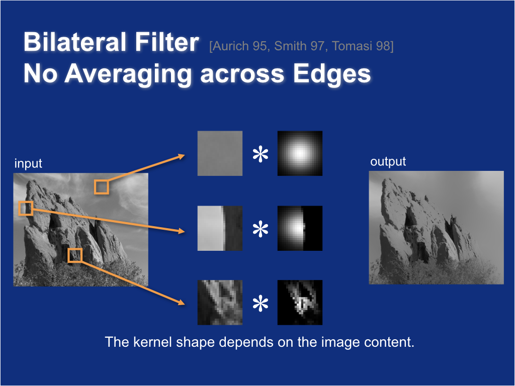
Bilateral filter: no averaging across edges
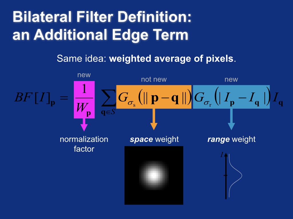
Bilateral filter definition
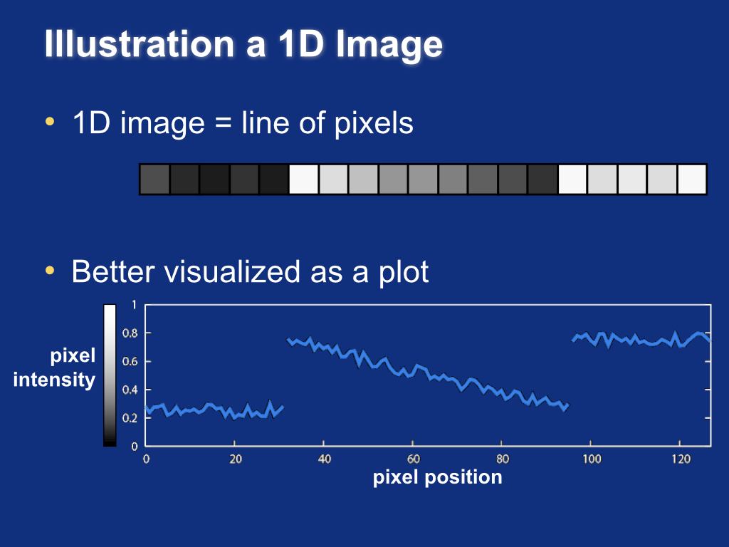
A 1D example
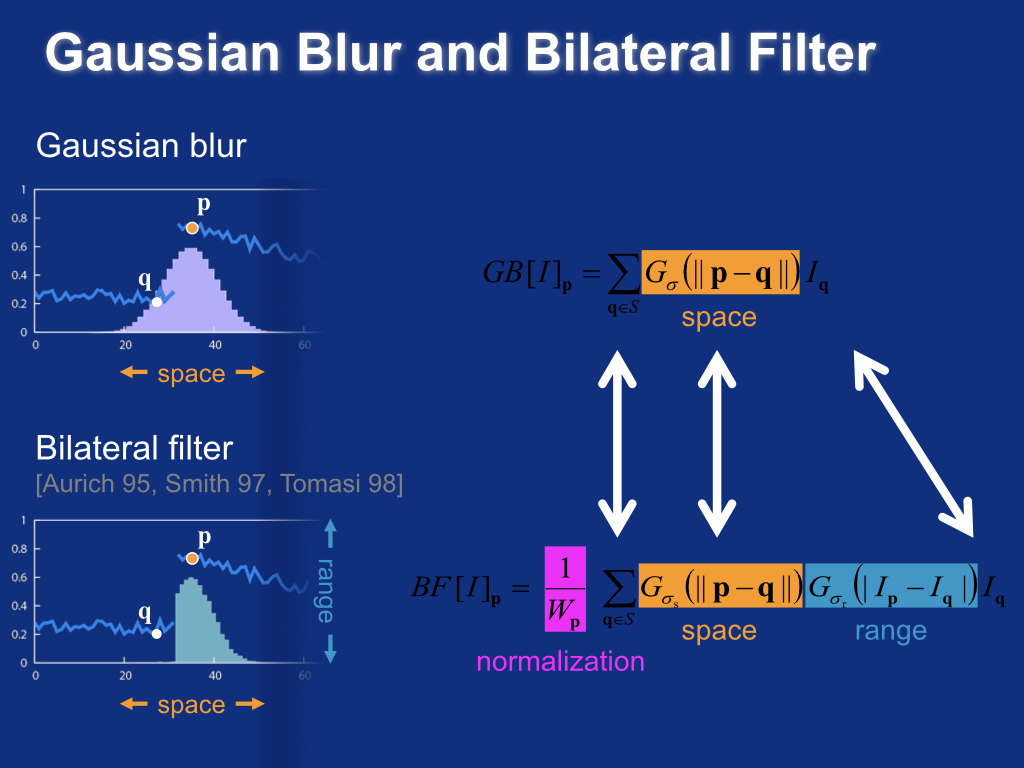
Gaussian blur and bilateral filter
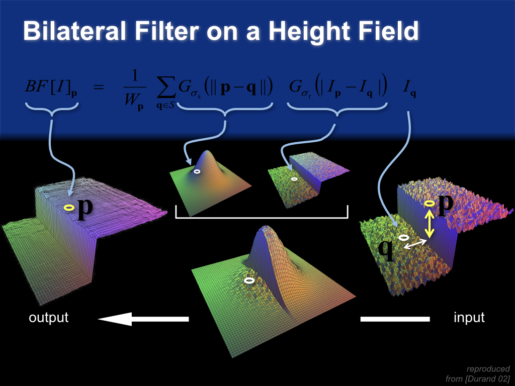
Bilateral filter on a height field
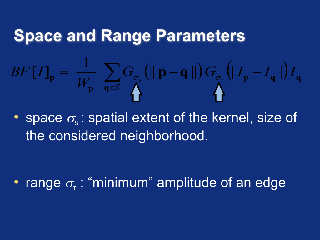
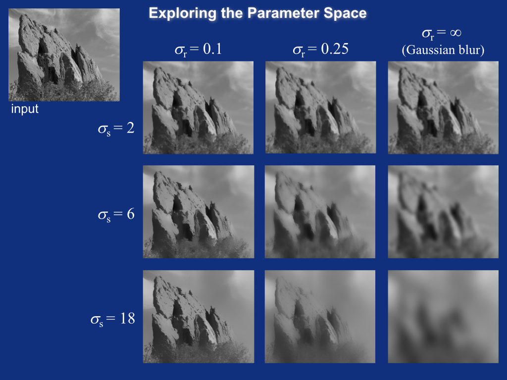
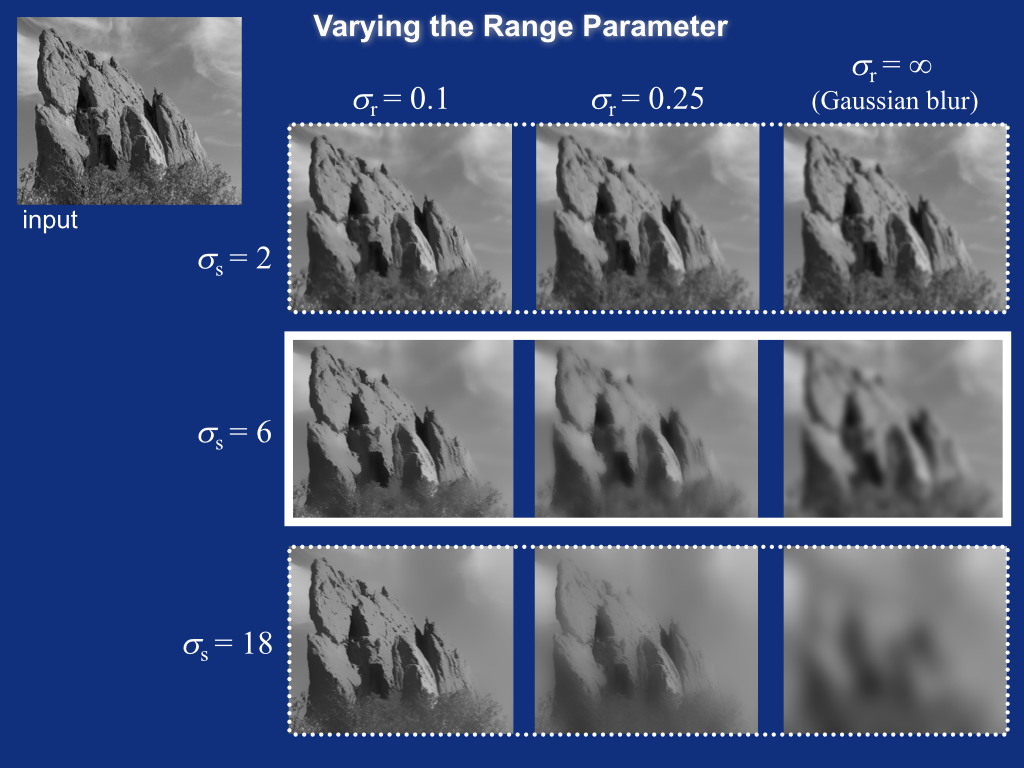
Space and range parameters
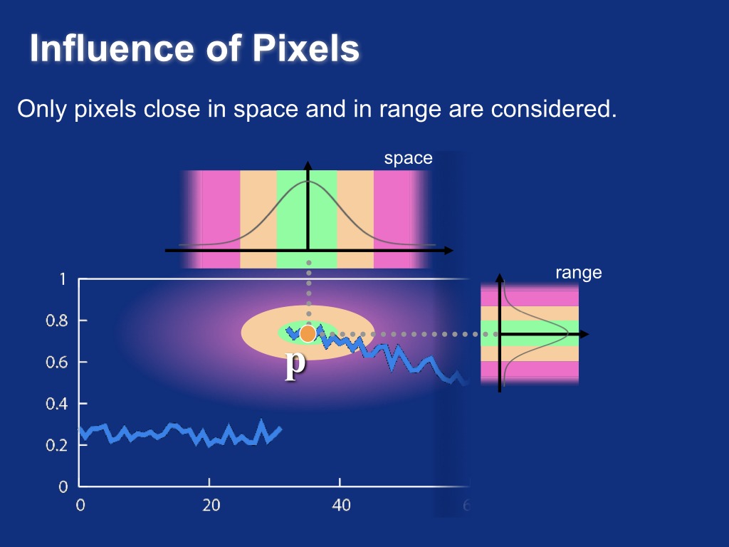
Influence of pixels
Exploring the parameter space
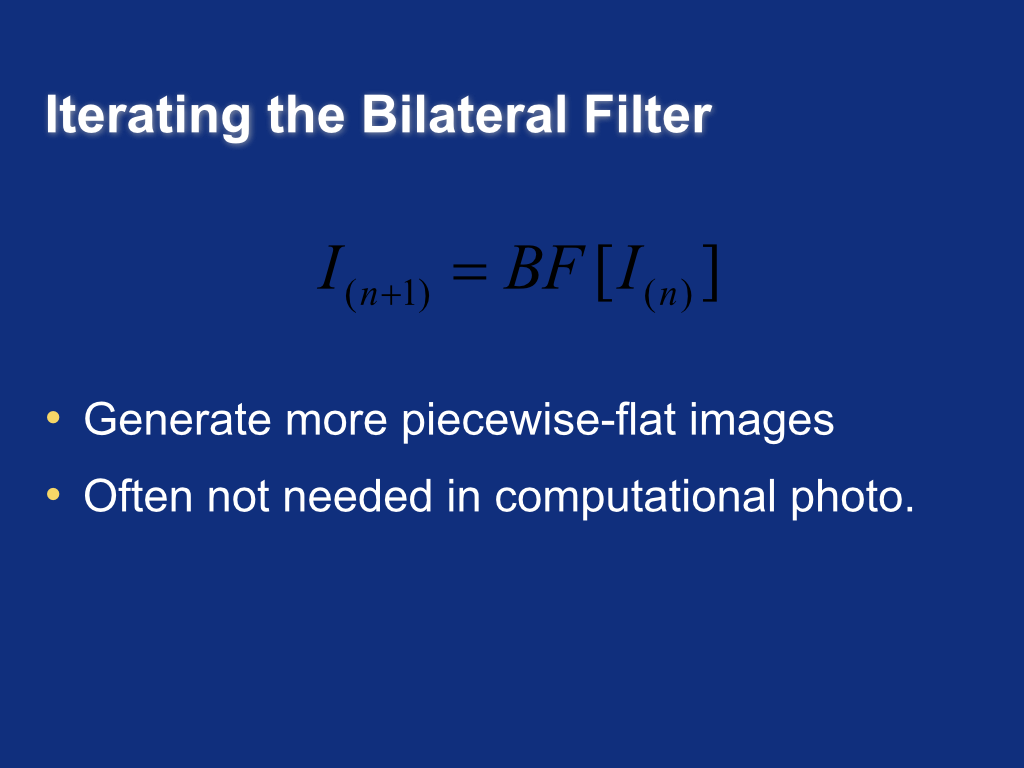
Iterating the bilateral filter
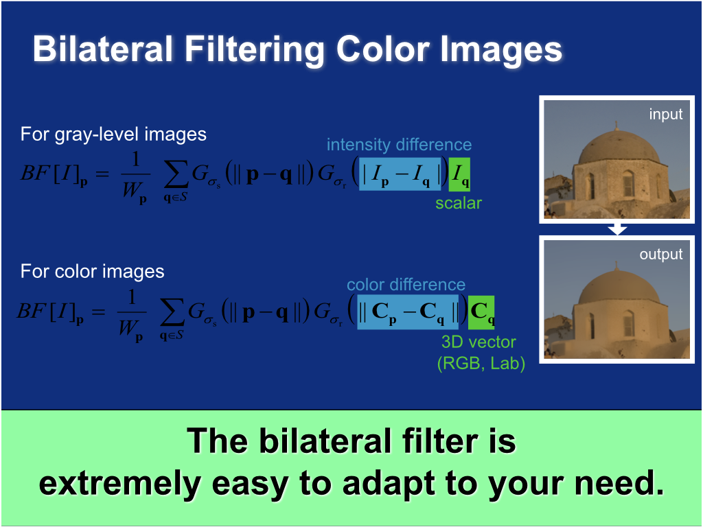
Bilateral filtering color images
Computational considerations