Local features

Faisal Qureshi
Professor
Faculty of Science
Ontario Tech University
Oshawa ON Canada
http://vclab.science.ontariotechu.ca

Copyright information

© Faisal Qureshi

License

This work is licensed under a Creative Commons Attribution-NonCommercial 4.0 International License.

Lesson Plan

• Characteristics of a good local feature
• Raw patches as local features
• SIFT descriptor
• Feature detection and matching in OpenCV
• Blob detection
• MSER in OpenCV
• Applications of local features

Motivation

Consider image stitching. It requires that we find corresponding "locations" in two images. Given these corresponding locations, we can compute homography, which would allow us to stitch the two images to construct a panorama.

Review: Characteristics of a Good Feature

• Repeatability — feature is invariant to geometric, lighting, etc. changes
• Saliency or distinctiveness
• Compactness — efficiency, many fewer features than the number of pixels in the image
• Locality — robustness to clutter and occlusion, a feature should only occupy a small area of an image

Repeatability

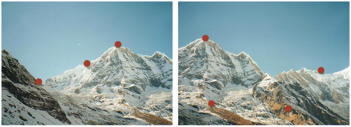
We need to find at least some of the same points in two images to any chance of finding true matches. There is little chance that we can find corresponding locations given the following two images.

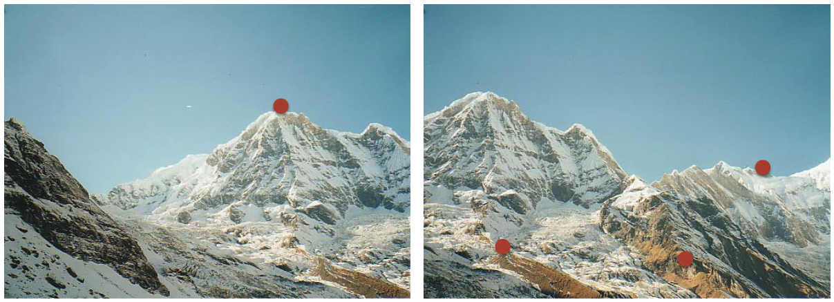
Detection process run independently on two images should return at least some of the corresponding locations as seen below.

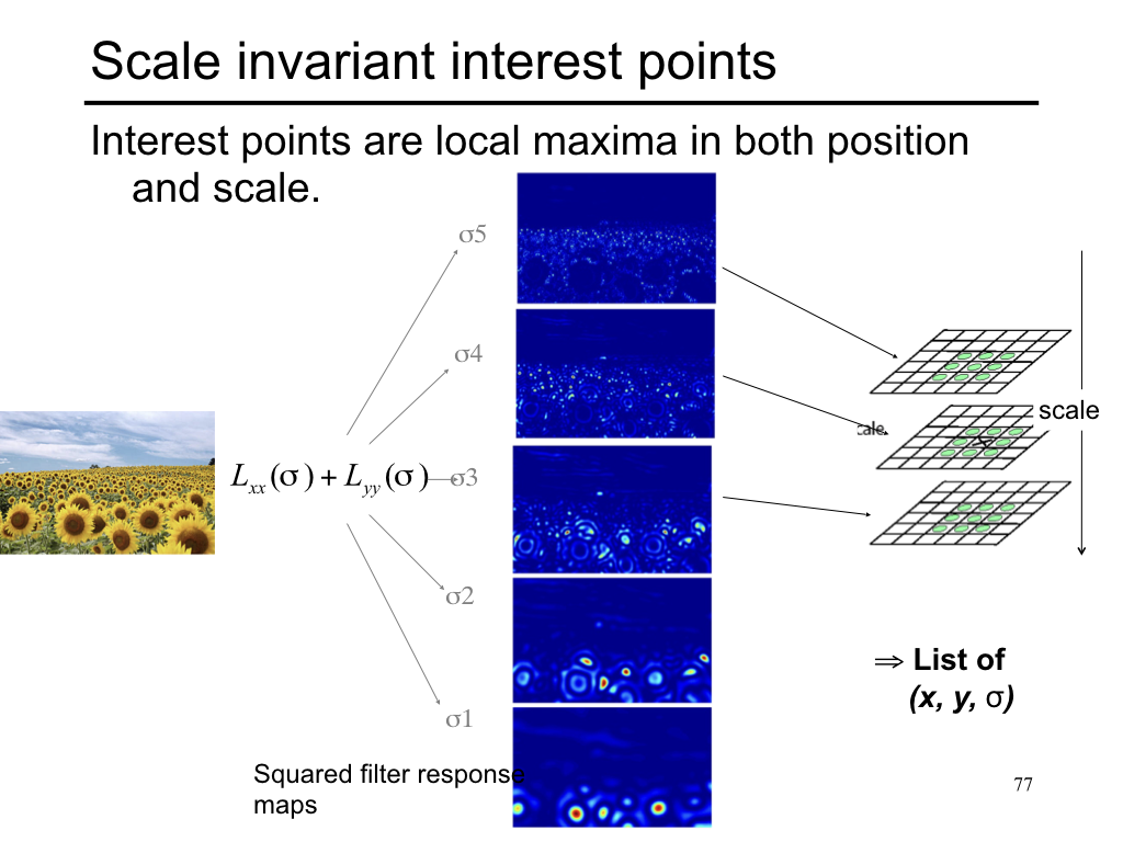
Recall that we have attempted to address this issue by interest point detection. These are locations in the image that are (somewhat) "invariant" to geometric and photometric changes. Specifically, we identified corner locations as those that are covariant to translation and rotation and partially invariant to changes in intensity. Recall also that corner detection is not invariant to changes in scale.

Observation 1: identify interest points locations (say, through corner detection) and construct local features around these locations.

Interest point detectors

Available interest point detectors

• Hessian & Harris [Beaudet 78], [Harris 88]
• Laplacian, Difference of Gaussian (DoG) [Lindeberg 98], [Lowe 99]
• Harris-/Hessian-Laplace [Mikolajczyk & Schmid 01]
• Harris-/Hessian-Affine [Mikolajczyk & Schmid 04]
• Edge-based Region Detector (EBR) and (Intensity Extrema Based Region Detector) IBR [Tuytelaars & Van Gool 04]
• Maximally Stable Extremal Regions (MSER) [Matas 02]
• Salient Regions [Kadir & Brady 01]
• and many others

Which interst point detector should you choose?

What do you want it for?

• Precise localization in x-y: Harris
• Good localization in scale: DoG
• Flexible region shape: MSER

Best choice often application dependent

• Harris-/Hessian-Laplace/DoG work well for many natural categories
• MSER works well for buildings and printed things

Take home lesson

• There have been extensive evaluations/comparisons [Mikolajczyk et al., IJCV 05, PAMI 05]. Best to check these out and select the best interest point detector for your application.
• It is sometimes useful to use multiple detectors simultaneously to help with matching over a range of image categories

We will soon see that deep learning has revolutionized image feature construction. More on this later.

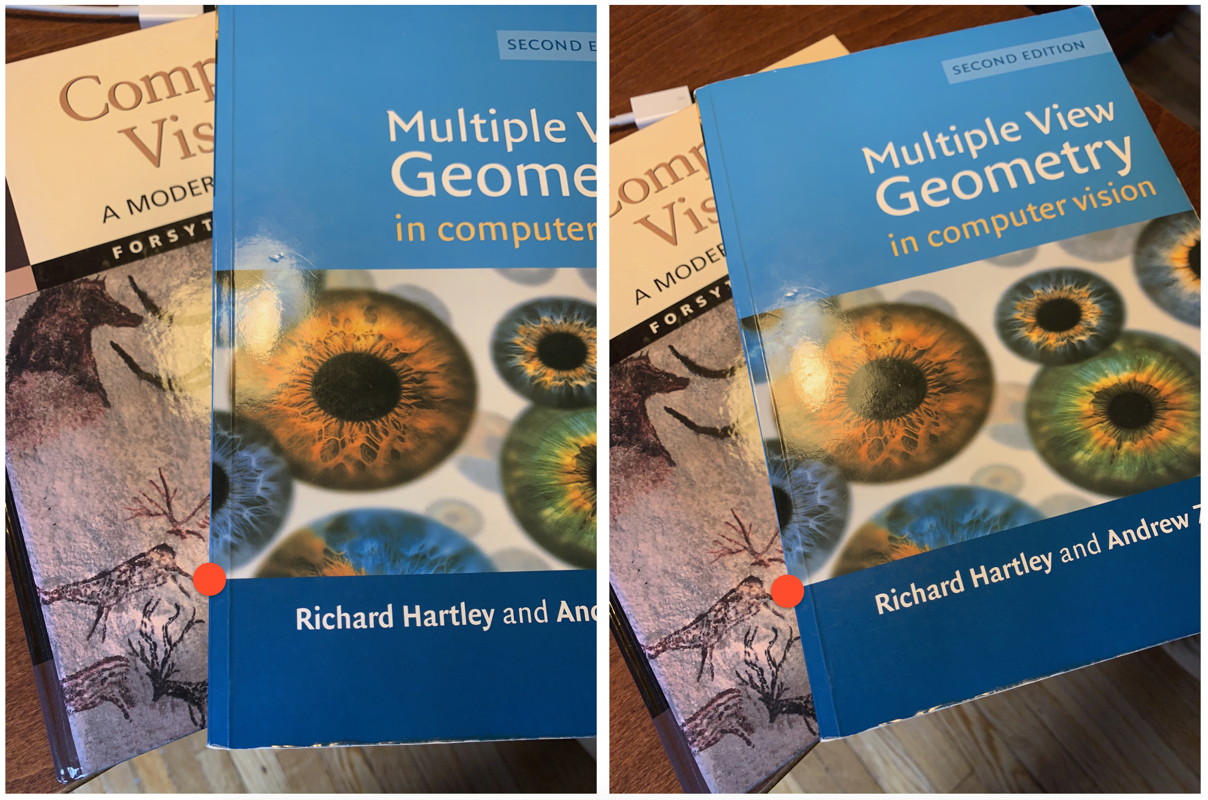
Saliency

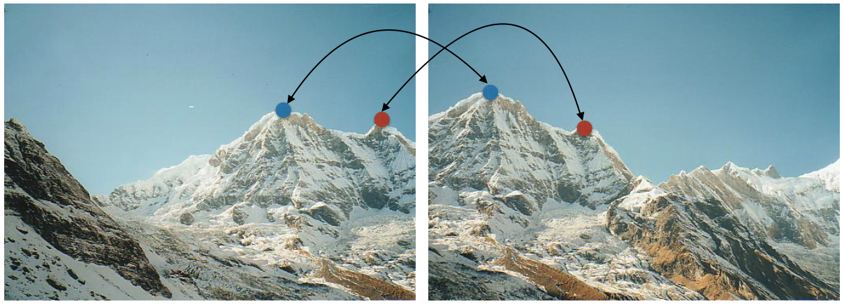
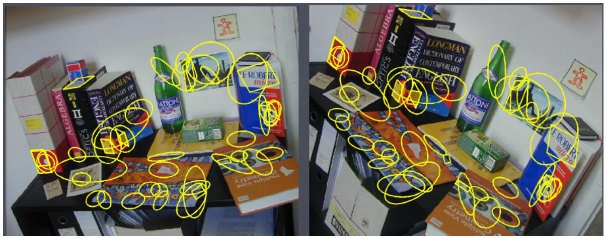
We want to reliably determine which location in one image goes with which location in the second image. The computed features should be invariant to geometric and photometric differences between the two images. Consider the following figure

Our task is to find the corresponding locations in the two images. This means that we need to figure out which of the two locations in the image on the right matches with the location shown in the image on the left.

Observation 2: compute descriptors that encode the area surrounding an interest point. These descriptors should be compact (for computational reasons), these should have local support, and these should have invariance properties with respect to geometric and photometric changes.

? Why do we want to encode local region around an interest point. Why not encode the entire image?

Local feature descriptors

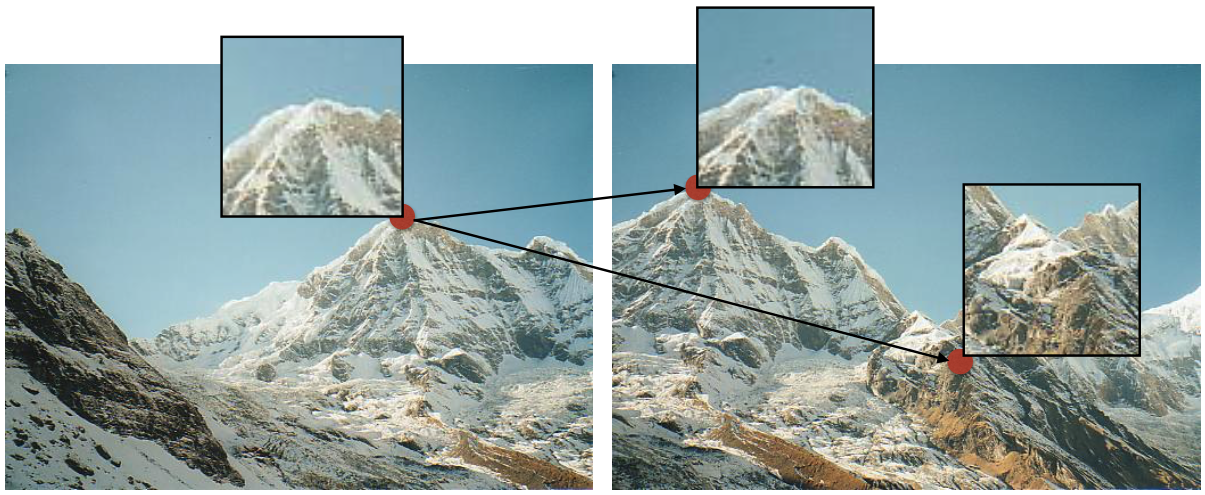
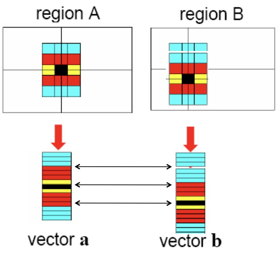
Encode area around interest points as vectors. We can then easily match these features to identify the corresponding locations between the two images. The following figure illustrates this idea. Here, local area around three interest point locations (one in the left image, and two in the right image) is encoded as $d$-dimensional vectors.

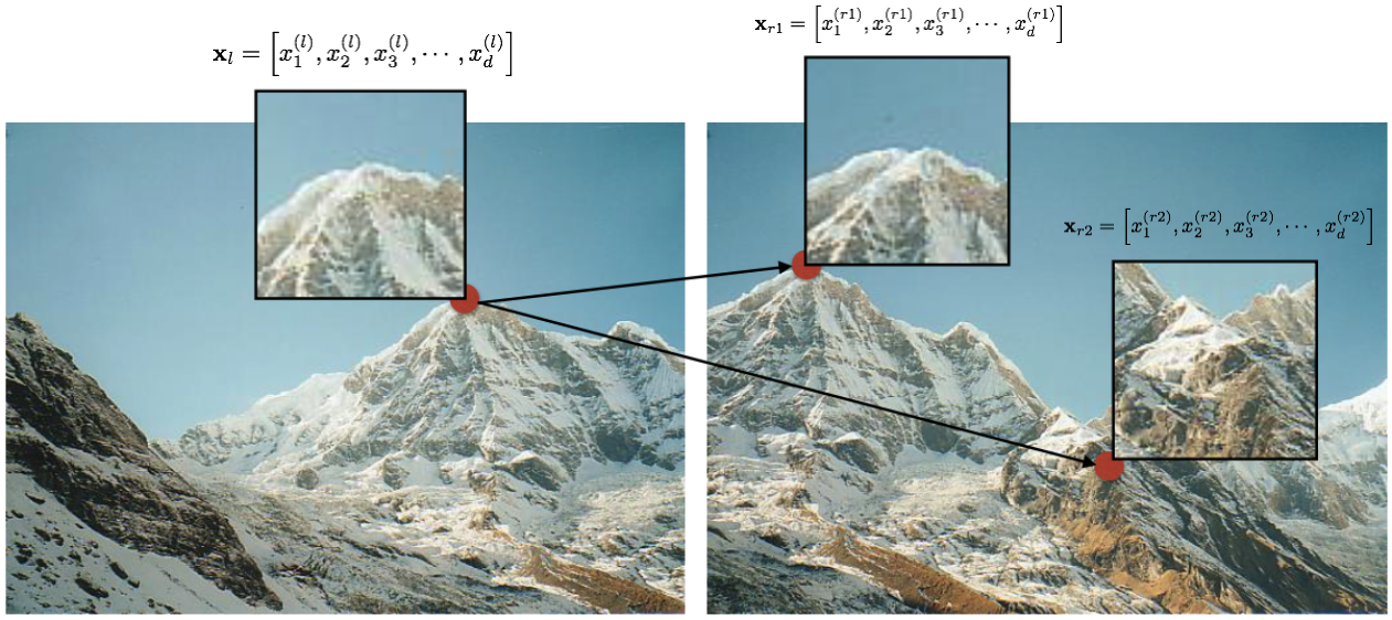
We can find the corresponding location by matching these $d$-dimensional vectors. There are many options for doing so. E.g., we can uses sum-of-squared differences (SSD) to match these vectors. Alternately, we can use cosine similarity. And there are many other techniques for matching vectors.

Computing local feature descriptors

Invariance to translation, rotation, and scale.

Invariance to changes in intensity and color.

(Figures courtesy T. Tuytelaars ECCV 2006 tutorial)

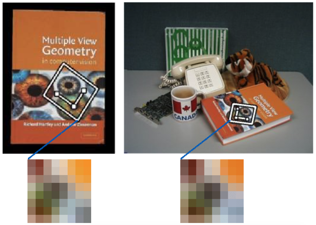
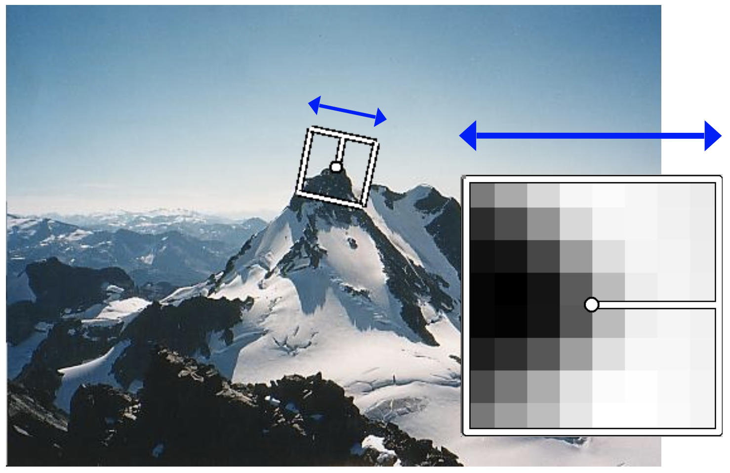
Raw patches as local descriptors

The simplest way to describe the neighborhood around an interest point is to write down the list of intensities to form a feature vector.
Consider the figure below.

The image patch around the interest point locations (depicted by the red circles) are as seen below.

Lets write down the list of intensities in these patches to form the feature vector

import numpy as np
import cv2 as cv
import matplotlib.pyplot as plt

left_patch = cv.imread('data/local-features-construction-2.jpg')
left_patch = cv.cvtColor(left_patch, cv.COLOR_BGR2RGB)
left_patch = cv.resize(left_patch, (32, 32), interpolation=cv.INTER_NEAREST)

right_patch = cv.imread('data/local-features-construction-1.jpg')
right_patch = cv.cvtColor(right_patch, cv.COLOR_BGR2RGB)
right_patch = cv.resize(right_patch, (32, 32), interpolation=cv.INTER_NEAREST)

plt.figure(figsize=(10,5))
plt.subplot(121)
plt.imshow(left_patch)
plt.subplot(122)
plt.imshow(right_patch);

Notice that listing intensities is very sensitiive to changes in rotation, scale, intensity, etc. These make poor feature descriptors.

Shift Invariant Feature Transform (SIFT) [Lowe 2004]

Description taken from various places, including https://sbme-tutorials.github.io/2019/cv/notes/7_week7.html

SIFT Pyramid

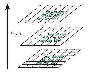
Construct SIFT pyramid, which consists of Octaves and Scales. Octaves are different levels of image resolutions (pyramids levels), and scales represent different scales of window in each octave level (different $\sigma$ of Gaussian window)

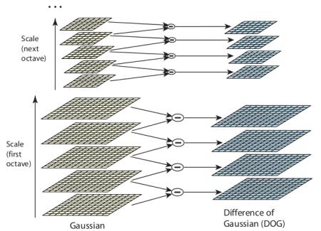
Key-point localization in scale

At each scale compare cornerness with neighbouring scales (upper and lower scales) and pick the scale with maximum cornerness value. Not all corners in an image are localized at the same scale.

Computing SIFT descriiptor

• Use image gradients instead of raw intensities
• Use histograms to bin pixels (gradients) within sub-patches according to their orientation.

• Use of image gradients provides partial invariance to changes in illumination
• Using subpatches maintains spatial structure.

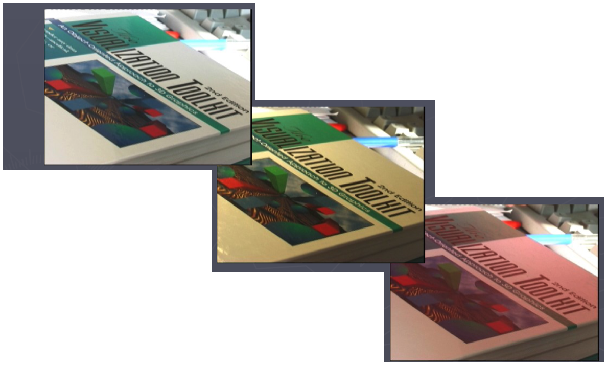
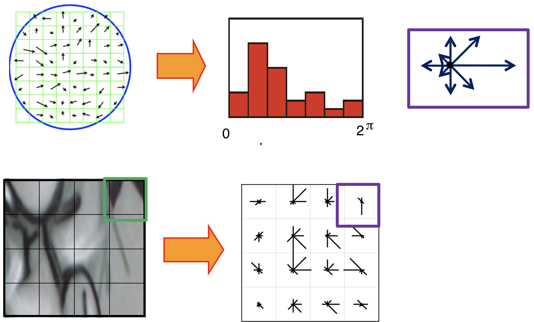
Achieving rotation invariance

Rotate patch according to its dominant gradient orientation. This puts the patches into a canonical orientation.

(Image from Matthew Brown.)

See below for how to find the dominant gradient orientation.

Computing SIFT descriiptor

• Use image gradients instead of raw intensities
• Use histograms to bin pixels (gradients) within sub-patches according to their orientation.

• Use of image gradients provides partial invariance to changes in illumination
• Using subpatches maintains spatial structure.

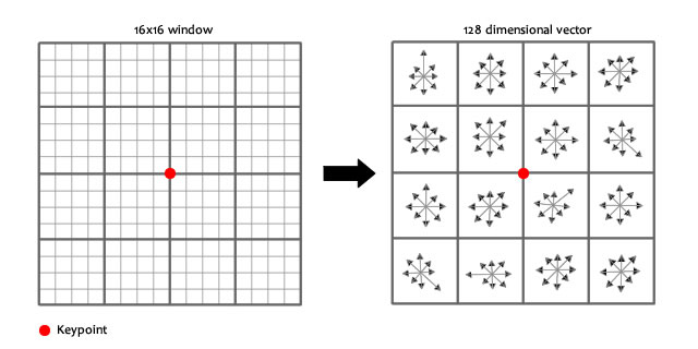
128-dimensional SIFT Descriptors

After localization of a key-point in our scale space. We can get its SIFT descriptor as follow

• Extract a $16 \times 16$ window centered by this point.
• Get gradient magnitude and multiply it by a $16 \times 16$ Gaussian window of $\sigma=1.5$
• Get gradient angle direction.
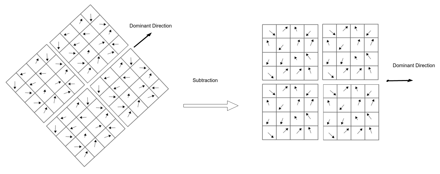
• Adjusting orientation (To be rotation invariant): get the gradient angle of the window and Quantize them to 36 values $(0, 10, 20, \cdots, 360)$
• Locate dominant corner direction which is most probable angle (angle with max value in 36 bit angle histogram) subtract dominant direction from gradient angle.
• For each block get magnitude weighted angle histogram and normalize it (divide by total gradient magnitudes). Here angles are quantized to 8 angles [0, 45, 90, … , 360] based on its relevant gradient magnitude i.e (histogram of angle 0 = sum(all magnitudes with angle 0)).

SIFT properties

• Extraordinarily robust matching technique
• Can handle changes in viewpoint of up to about 60 degree out of plane rotation
• Can handle significant changes in illumination

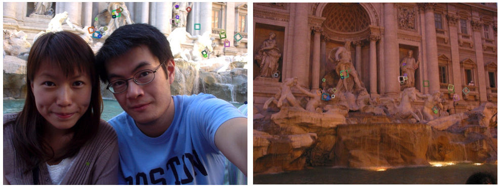
(Image from Steve Seitz)

• Fast and efficient—can run in real time

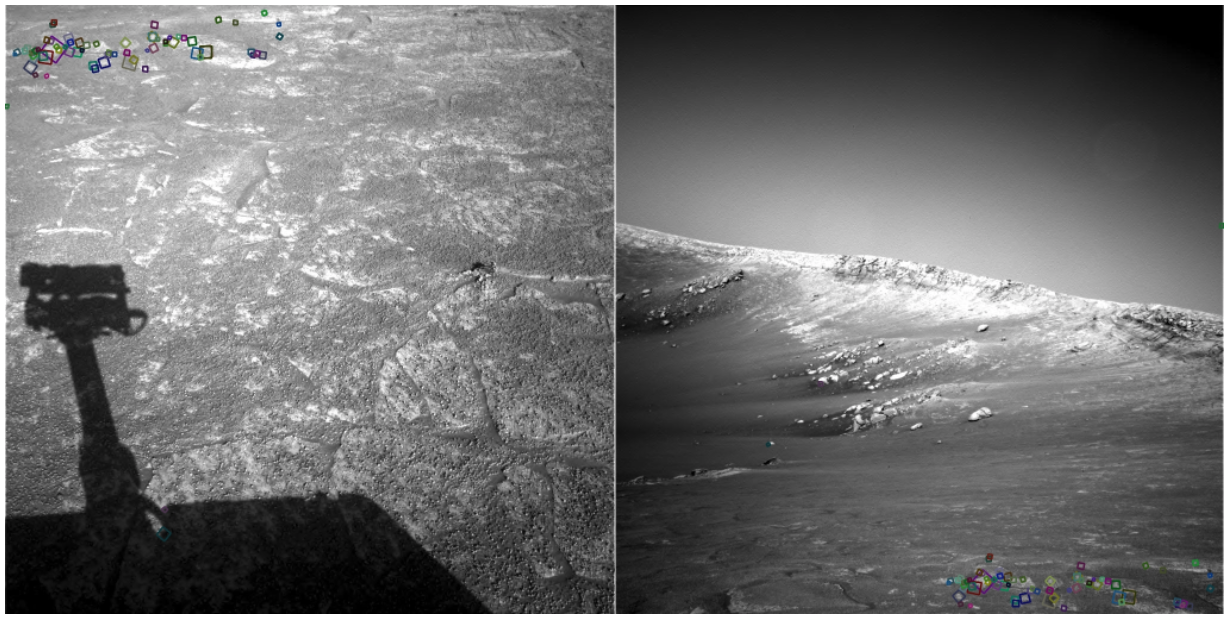
NASA Mars Rover images with SIFT feature matches. (Figure by Noah Snavely.)

SIFT summary

• Invariant to scale and rotation
• Partially invariant to illumination changes, camera viewpoint, occlusion, and clutter

SIFT Code

SIFT was initially included in OpenCV; however, it is no longer available. Since SIFT was patented. An option is to use VLfeat library, which includes a SIFT implementation. VLfeat currently doesn't have a "stable" Python biding. Still you are welcome to try it using pip install pyvlfeat.

Matching local features

Consider the figures below. "SIFT patches" are overlaid on the two images. Our goal is to generate candidate matches.

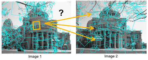
Classical feature descriptors, such as SIFT, SURF, etc., are usually compared and matched using the Euclidean distance (or L2-norm). Other techniques for matching these features are Cosine similarity, Earth Mover's Distance (also known as Wasserstein Distance), etc.

Distance computation in Python

Check out scipy.spatial.distance module for various methods for computing distance matrix for a collection of raw observation vectors stored in a rectangular array.

See here for more information.

Exercise 1

Compute Cosine and Euclidean distance matrix between three vectors $[1,0,0]$, $[0,1,0]$, $[1,1,0]$, and $[10,-2,1]$

Solution:

# %load solutions/local-features/solution-01.py
# Local features - Exercise 01

from scipy.spatial import distance
import numpy as np

a = np.array([1,0,0])
b = np.array([0,1,0])
c = np.array([1,1,0])
d = np.array([10,-2,1])

# Set up an m-by-n matrix, where m is the number of
# data items and n is the dimension
X = np.vstack((a,b,c,d))
#print(f'Shape of X is {X.shape}')

# D is condensed matrix
metric = ['cosine', 'euclidean']
i = 0
D = distance.pdist(X, metric[i])

# Lets convert it into square form
print(f'{metric[i]} similarity:')
print(distance.squareform(D))

cosine similarity:
[[0.         1.         0.29289322 0.02409993]
 [1.         0.         0.29289322 1.19518001]
 [0.29289322 0.29289322 0.         0.44794755]
 [0.02409993 1.19518001 0.44794755 0.        ]]

From distance to similarity

How do we convert distance values to similarity values. For cosine distance, simply subtract cosine distance from 1.0. In general if your distance metric returns values between 0 and 1, then you can use this trick.

Exercise 2

Compute Cosine similarity matrix between $[1,0,0]$, $[0,1,0]$, $[1,1,0]$, and $[10,-2,1]$

Solution:

# %load solutions/local-features/solution-02.py
# Local features - Exercise 02

from scipy.spatial import distance
import numpy as np

a = np.array([1,0,0])
b = np.array([0,1,0])
c = np.array([1,1,0])
d = np.array([10,-2,1])

# Set up an m-by-n matrix, where m is the number of
# data items and n is the dimension
X = np.vstack((a,b,c,d))
#print(f'Shape of X is {X.shape}')

# D is condensed matrix
metric = ['cosine', 'euclidean']
i = 0
D = distance.pdist(X, metric[i])

# Lets convert it into square form
print(f'{metric[i]} similarity:')
print(1.0 - distance.squareform(D))

cosine similarity:
[[ 1.          0.          0.70710678  0.97590007]
 [ 0.          1.          0.70710678 -0.19518001]
 [ 0.70710678  0.70710678  1.          0.55205245]
 [ 0.97590007 -0.19518001  0.55205245  1.        ]]

Gaussian kernel to convert distance to similarity

For other distances, we can use, say, a Gaussian kernel as follows:

$$ K(d) = \exp \left( \frac{d^2} {2 \sigma^2} \right), $$

where $d$ is the distance between two vectors $\mathbf{x}_1$ and $\mathbf{x}_2$. $\sigma$ is a tuning (or scaling) parameter. If $\sigma$ is high, $K(d)$ will be close to $1$ (i.e., high similarity) for large values of $d$. If $\sigma$ is small, even a small $d$ will reduce the similarity scores for the two vectors.

Exercise 3

Compute similarity matrix between $[1,0,0]$, $[0,1,0]$, $[1,1,0]$, and $[10,-2,1]$. Assume Euclidean distance metric.

Solution:

# %load solutions/local-features/solution-03.py
# Local features - Solution 03

from scipy.spatial import distance
import numpy as np

a = np.array([1,0,0])
b = np.array([0,1,0])
c = np.array([1,1,0])
d = np.array([10,-2,1])

# Set up an m-by-n matrix, where m is the number of
# data items and n is the dimension
X = np.vstack((a,b,c,d))
#print(f'Shape of X is {X.shape}')

# D is condensed matrix
metric = ['cosine', 'euclidean']
i = 1
D = distance.squareform(distance.pdist(X, metric[i]))
print('Distance:\n', D)

# Lets convert it into square form
sigma = 0.0001
scaling = 2 * (sigma ** 2)

print(f'{metric[i]} similarity:')
np.set_printoptions(formatter={'float': lambda x: "{0:0.1e}".format(x)})
S = np.exp(-D**2 / (scaling))
print('Similarity:\n', S)
np.set_printoptions() # To not mess with other printing

Distance:
 [[ 0.          1.41421356  1.          9.2736185 ]
 [ 1.41421356  0.          1.         10.48808848]
 [ 1.          1.          0.          9.53939201]
 [ 9.2736185  10.48808848  9.53939201  0.        ]]
euclidean similarity:
Similarity:
 [[1.0e+00 0.0e+00 0.0e+00 0.0e+00]
 [0.0e+00 1.0e+00 0.0e+00 0.0e+00]
 [0.0e+00 0.0e+00 1.0e+00 0.0e+00]
 [0.0e+00 0.0e+00 0.0e+00 1.0e+00]]

Wasserstein distance

Wasserstien distance is computed between two probability distributions (below represented as histograms). Check out scipy.stats module for methods for computing Wasserstien distance.

from scipy.stats import wasserstein_distance
wasserstein_distance([0, 1, 3], [5, 6, 8])

np.float64(5.0)

Hamming distance

We now also have binary feature descritors, such as ORB, BRISK, which are matched using Hamming distance.

$$ d_{\mathrm{hamming}} (\mathbf{a}, \mathbf{b}) = \sum_{i=0}^{n-1} (a_i \oplus b_i) $$

Aside:

• SIFT descriptors represent the histogram of oriented gradient in a neighbourhood
• SURF descriptors represent the histogram of of the Haar wavelet response in a neighborhood
• See here) for more information about Binary Robust Independent Elementary Features (BRIEF)
• Oriented Fast and Rotated Brief (ORB) [Ethan Rublee et al. 2011]

Bruteforce matching

Compare them all, take the closest (or closest $k$, or within a thresholded distance).

import numpy as np
import cv2 as cv
import matplotlib.pyplot as plt

img1 = cv.imread('data/box.png',cv.IMREAD_GRAYSCALE)          
img2 = cv.imread('data/box_in_scene.png',cv.IMREAD_GRAYSCALE) 
print(img1.shape)

(223, 324)

orb = cv.ORB_create()
kp1, des1 = orb.detectAndCompute(img1, None) # locations and descriptor
kp2, des2 = orb.detectAndCompute(img2, None)

bf = cv.BFMatcher(cv.NORM_HAMMING, crossCheck=True)
matches = bf.match(des1, des2)
matches = sorted(matches, key = lambda x:x.distance)

img3 = cv.drawMatches(img1, kp1, img2, kp2, matches[:10], None, flags=cv.DrawMatchesFlags_NOT_DRAW_SINGLE_POINTS)

plt.figure(figsize=(10,10))
plt.imshow(img3)
plt.show()

KDTree data structure

See here for more information.

Solution:

# %load solutions/local-features/kdtree.py
# Local Features - kdtree.py

import numpy as np
from scipy.spatial import KDTree

rng = np.random.RandomState(0)
X = rng.random_sample((10, 3))
print(X)
T = KDTree(X, leafsize=3)
distance, index = T.query(X[0,:]) # Try to perturb the query vector +[0.01,0.01,0]
print(f'distance={distance}, data={X[index,:]}')

[[0.5488135  0.71518937 0.60276338]
 [0.54488318 0.4236548  0.64589411]
 [0.43758721 0.891773   0.96366276]
 [0.38344152 0.79172504 0.52889492]
 [0.56804456 0.92559664 0.07103606]
 [0.0871293  0.0202184  0.83261985]
 [0.77815675 0.87001215 0.97861834]
 [0.79915856 0.46147936 0.78052918]
 [0.11827443 0.63992102 0.14335329]
 [0.94466892 0.52184832 0.41466194]]
distance=0.0, data=[0.5488135  0.71518937 0.60276338]

Ambiquous matches

Lets consider SSD metric for finding matches. How do we threshold on SSD? One approach is to compute the ratio of the distance to best match to distance to the second best match. If this ratio is low, the best match is a good candidate. If this ratio is high, then the best match could be an ambiguous match.

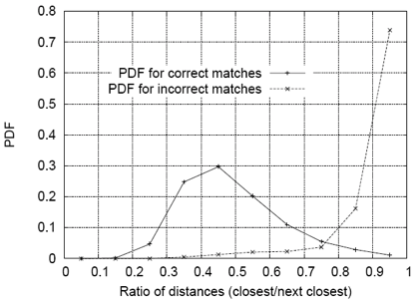
(Figure from Lowe 2004)

FLANN matching

Check this for more information.

(From OpenCV documentation) FLANN stands for Fast Library for Approximate Nearest Neighbors. It contains a collection of algorithms, such as KDTree, Locality Sensitive Hashing, etc., optimized for fast nearest neighbor search in large datasets and for high dimensional features. It works more faster than BFMatcher for large datasets.

For OpenCV implementation, possible values are:

• FLANN_INDEX_LINEAR = 0
• FLANN_INDEX_KDTREE = 1
• FLANN_INDEX_KMEANS = 2
• FLANN_INDEX_COMPOSITE = 3
• FLANN_INDEX_KDTREE_SINGLE = 4
• FLANN_INDEX_HIERARCHICAL = 5
• FLANN_INDEX_LSH = 6
• FLANN_INDEX_SAVED = 254
• FLANN_INDEX_AUTOTUNED = 255

import numpy as np
import cv2 as cv
import matplotlib.pyplot as plt

img1 = cv.imread('data/box.png',cv.IMREAD_GRAYSCALE)          
img2 = cv.imread('data/box_in_scene.png',cv.IMREAD_GRAYSCALE) 

orb = cv.ORB_create()
kp1, des1 = orb.detectAndCompute(img1, None) # locations and descriptor
kp2, des2 = orb.detectAndCompute(img2, None)

FLANN_INDEX_LSH = 6
index_params = dict(algorithm = FLANN_INDEX_LSH, table_number = 6)
search_params = dict(checks=50)
flann = cv.FlannBasedMatcher(index_params, search_params)

matches = flann.knnMatch(des1, des2, k=2)

good = []
for match in matches:
    if len(match) < 2: continue
    m, n = match[0], match[1]
    if m.distance < 0.75*n.distance:
        good.append([m])

img3 = cv.drawMatchesKnn(img1, kp1, img2, kp2, good, None, flags=cv.DrawMatchesFlags_NOT_DRAW_SINGLE_POINTS)
plt.figure(figsize=(10,10))
plt.imshow(img3)
plt.show()

Blob detection

Edge detection review

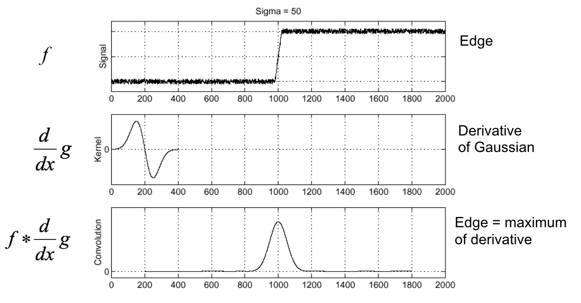
(Figure from Steve Seitz).

Second derivative of Gaussian (Laplacian)

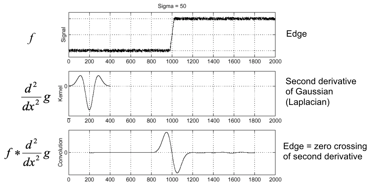
(Figure from Steve Seitz).

From edges to blobs

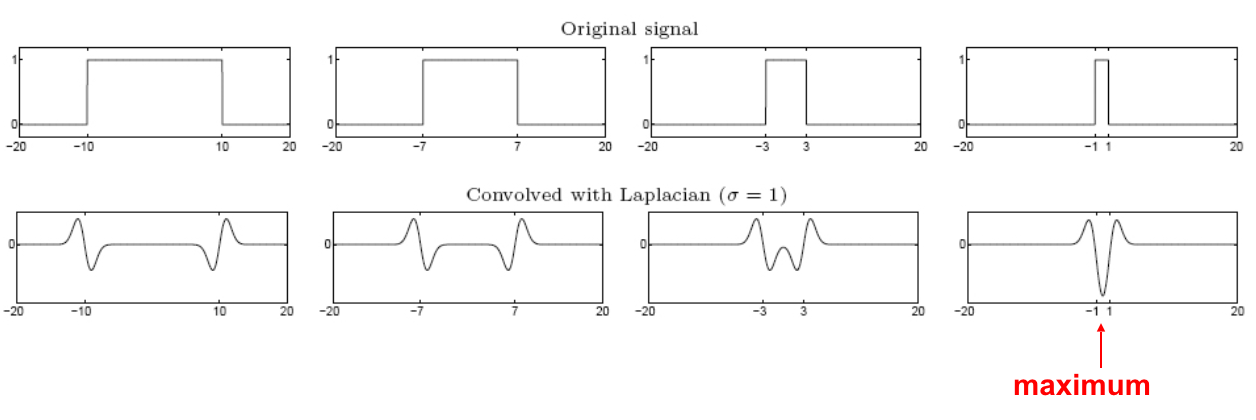
(Figure from Lana Lazebnik).

• Edge = ripple
• Blob = superposition of two ripples
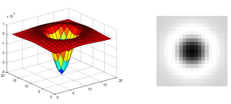
• Spatial selection: the magnitude of the Laplacian response will achieve a maximum at the center of the blob, provided the scale of the Laplacian is "matched" to the scale of the blob

Blob detection in 2D

Laplacian of Gaussian is circularly symmetric operator for blob detection in 2D.

$$ \nabla^2 g = \frac{\partial^2 g}{\partial x^2} + \frac{\partial^2 g}{\partial y^2} $$

(Figure from Lana Lazebnik).

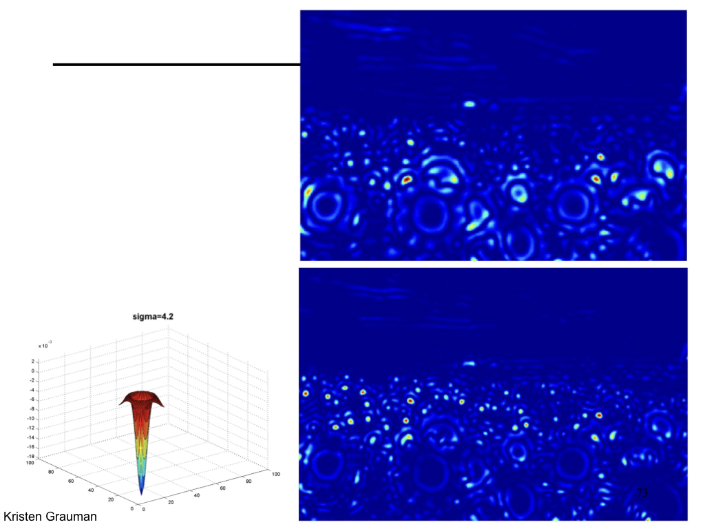
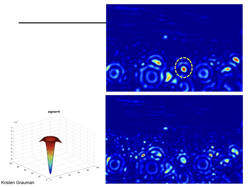
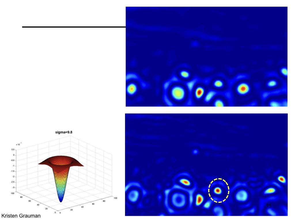
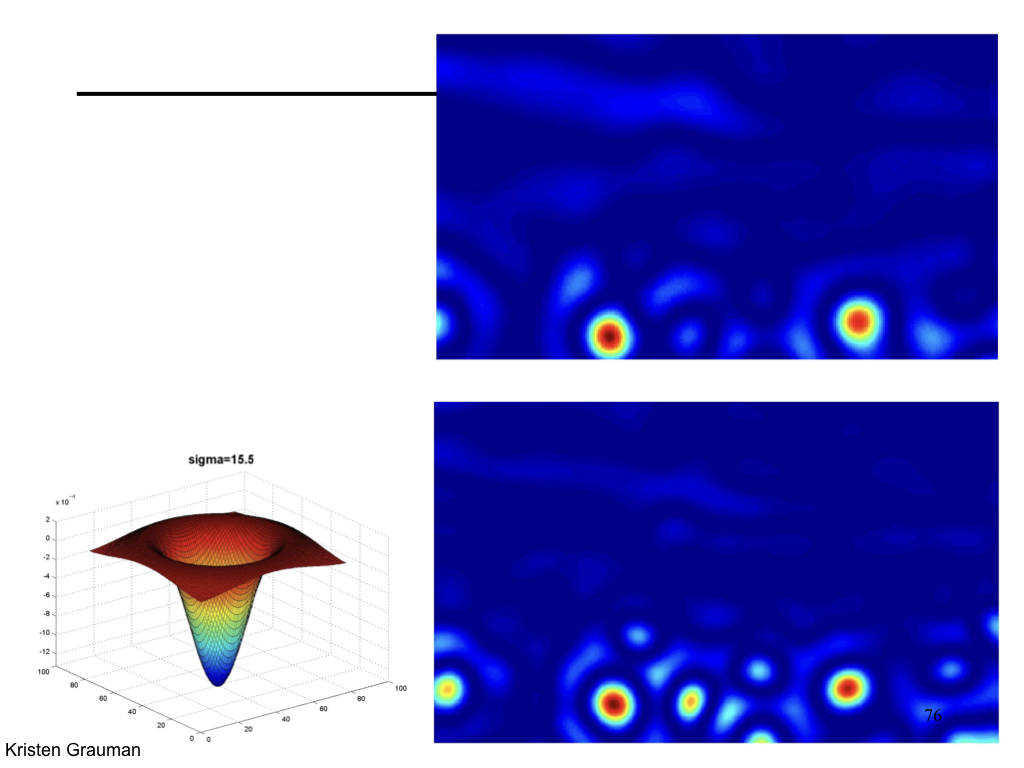
Characteristic scale

We define the characteristic scale as the scale that produces peak of Laplacian response.

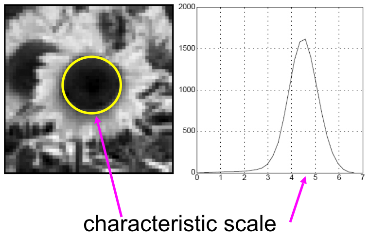
(Figure from Lana Lazebnik).

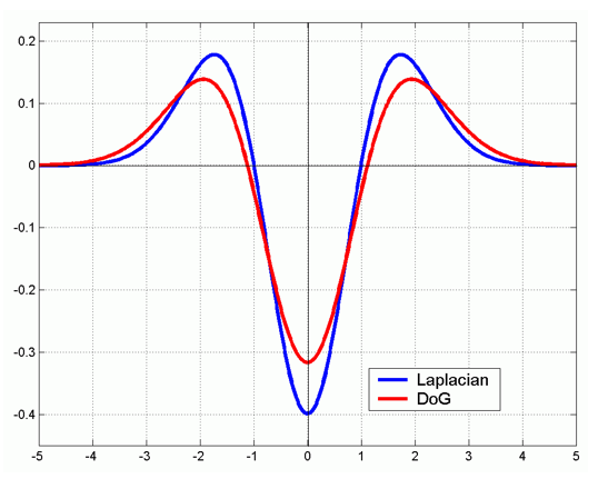
Difference of Gaussian

We can approximate Laplacian as Difference of Gaussian (DOG), which much more efficient to compute.

Blob detection example in OpenCV

The relevant parameters are described below:

• Area: filter the blobs based on size
• Circularity: a measure of how close the blob is to a circle. Circularity is defined by $\frac{4 \pi\ \mathrm{area}}{\mathrm{parameter}}$.
• Convexity: the ratio of area of the blob and the are of its convex hull. Convexity values lie between $0$ and $1$, inclusive.
• Inertia: the measure of "ellipseness" of a shape. A circle has inertia of $1$ and a line has inertia of $0$. The inertia of an ellipse lies somewhere between $0$ and $1$.

import cv2 as cv
import numpy as np
import matplotlib.pyplot as plt

filename = "data/butterfly.jpg"
#filename = "data/BlobTest.jpg"
im = cv.imread(filename)
im = cv.cvtColor(im, cv.COLOR_BGR2RGB)

params = cv.SimpleBlobDetector_Params()
params.minThreshold = 10 # Change thresholds
params.maxThreshold = 250
params.filterByArea = False # Filter by Area.
params.minArea = 100
params.filterByCircularity = False # Filter by Circularity
params.minCircularity = 0.1
params.filterByConvexity = False # Filter by Convexity
params.minConvexity = 0.9
params.filterByInertia = False # Filter by Inertia
params.minInertiaRatio = 0.9
detector = cv.SimpleBlobDetector_create(params)

keypoints = detector.detect(im)

im_with_keypoints = cv.drawKeypoints(im, keypoints, np.array([]), (255,0,0), cv.DRAW_MATCHES_FLAGS_DRAW_RICH_KEYPOINTS)

plt.figure(figsize=(15,15))
plt.imshow(im_with_keypoints);

Maximally Stable Extremal Region (MSER)

MSER detects homogeneous regions. We can use the centroids of these regions as keypoint locations.

MSER are affine invariant, which means that image skew or warping doesn't effect these. In addition, MSER are also "partially" invariant to changes in image intensity. In addition, MSER have the followign useful properties:

• Multi-scale detection without any smoothing involved, both fine and large structure is detected
• Only regions whose support is nearly the same over a range of thresholds is selected, which leads to stability
• The set of all extremal regions can be enumerated in worst-case $\mathcal{O} (n)$, where $n$ is the number of pixels in the image.
• Covariance to adjacency preserving (continuous) transformation $T: D \to D$

For more information, check this wiki article.

MSER in OpenCV

#im = cv.imread('data/apple.jpg');
im = cv.imread('data/box.png');
im = cv.cvtColor(im, cv.COLOR_BGR2RGB)
vis = im.copy()

mser = cv.MSER_create()
regions, bboxes = mser.detectRegions(im)

hulls = [cv.convexHull(p.reshape(-1, 1, 2)) for p in regions]
cv.polylines(vis, hulls, 1, (255, 0, 255), 1)
plt.figure(figsize=(10,10))
plt.imshow(vis);

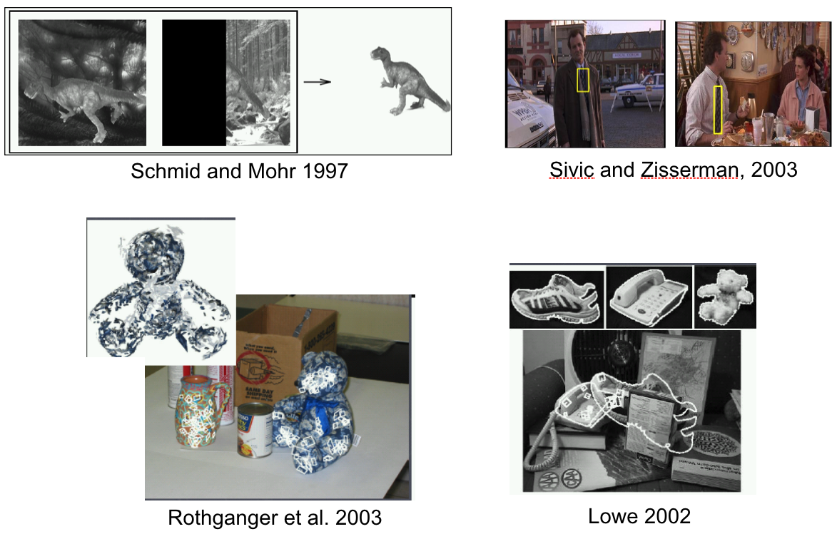
Applications of local invariant features

• Wide baseline stereo
• Motion tracking
• Panoramas
• Mobile robot navigation
• 3D reconstruction
• Recognition

Panoramas

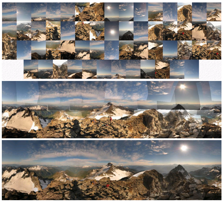
(Figure from UBC autostich)

Wide base-line stereo

(Image from T. Tuytelaars ECCV 2006 tutorial)

Object recogniton

(Figure from Kristen Grauman)