Interest Point Detection
Faisal Qureshi
Professor
Faculty of Science
Ontario Tech University
Oshawa ON Canada
http://vclab.science.ontariotechu.ca
Copyright information
© Faisal Qureshi
License

This work is licensed under a Creative Commons Attribution-NonCommercial 4.0 International License.
import numpy as np
import scipy as sp
from scipy import signal
import cv2 as cv
import matplotlib.pyplot as plt
import matplotlib as mpl
from matplotlib import cm
from matplotlib.ticker import LinearLocator, FormatStrFormatter
Lesson Plan
- Uses of interest point detection
- Interest point detection and its relationship to feature descriptors and feature matching
- Interest point detection
- Corner detection
This notebook focuses on interest point detection. We leave feature descriptors and feature matching for an other time.
Uses
- Image alignment
- 3D reconstruction
- Tracking
- Object recognition
- Image retrieval
- Navigation (or mapping)
Example: Image (or object) matching
Step 1: Detect interest points locations
Step 2: Compute feature descriptors around interest point locations
Step 3: Use descriptor matching for finding corresponding locations in two or more images
Characteristics of a Good Feature
Repeatability
Invariance to geometric, lighting, etc. changes
Saliency or distinctiveness
Invariance to geometric and photometric differences between two images
Compactness (Efficiency)
Many fewer features than the number of pixels in the image
Locality
Robustness to clutter and occlusion, a feature should only occupy a small area of an image
Detecting Interest Point Locations
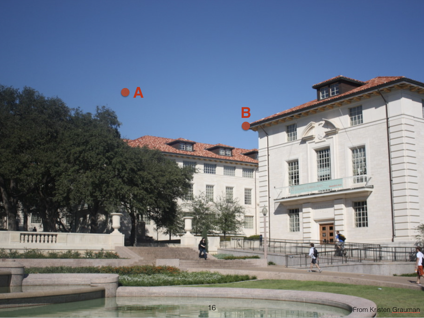
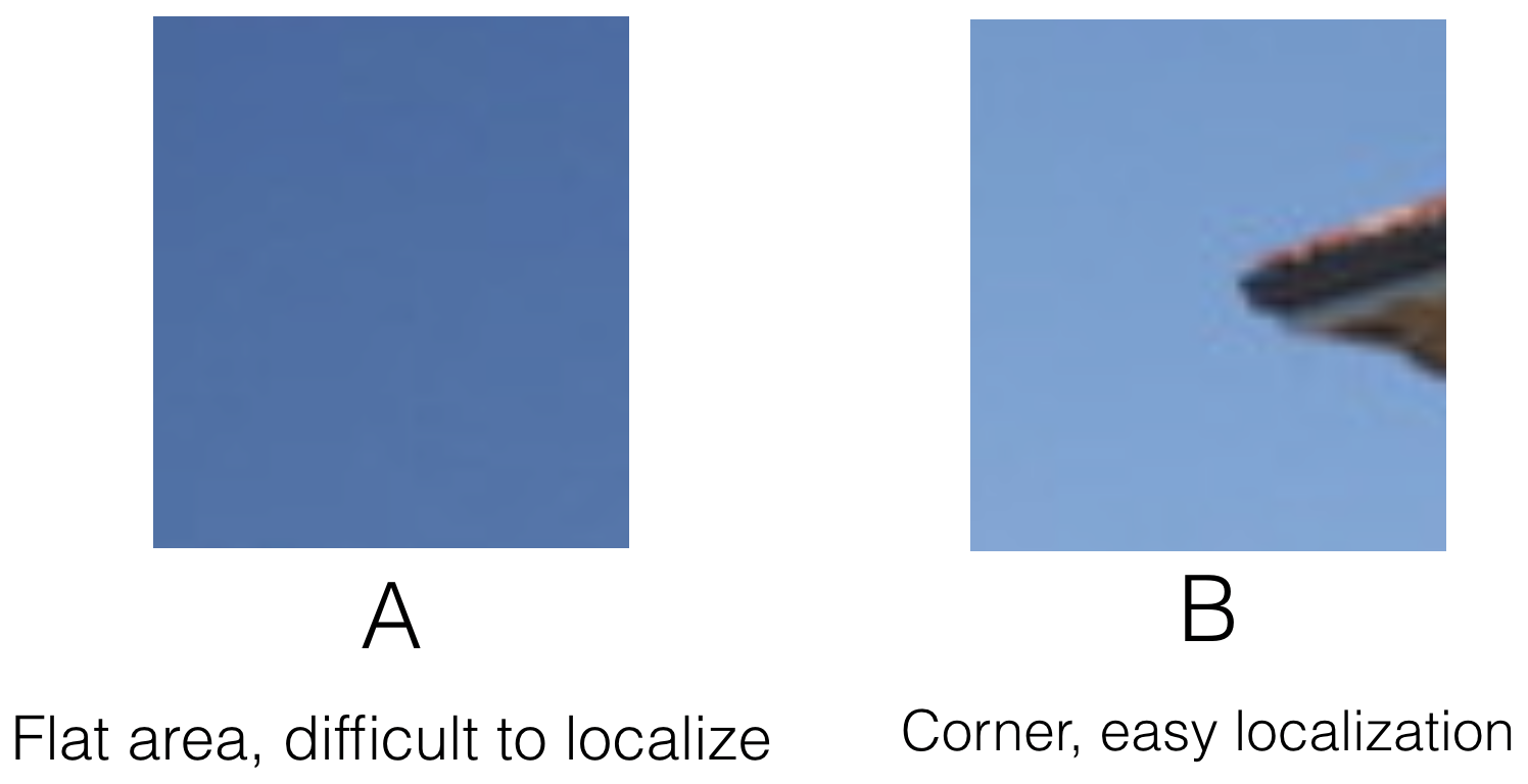
Which is a better location for an interest point: A or B?
Corner Detection
In the following figure: (left) represents a flat region where there is no change is observed in any direction as we move the window; (middle) represents an edge region where change is observed in one direction only as we move the window; and (right) represents a corner region where change is observed in two direction as we move the window.
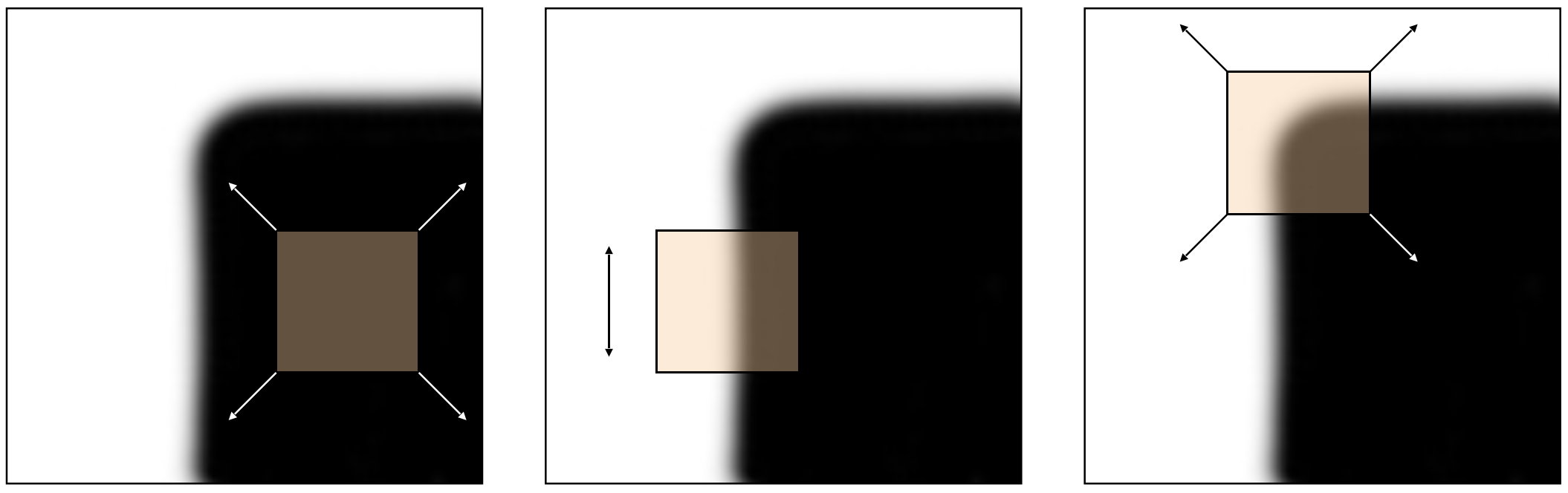
Notice that unlike flat and edge regions, corners can be "easily" localized. Recall that this is one of the requirements for interest point detection.
In the remaining of this section, we will focus on corner detection.
Quantifying neighbourhood structure
We can capture the change in appearance as we move the window around as follows:
$$ E(u,v) = \sum_{x,y} w(x,y) [I(x+u, y+v) - I(x,y)]^2 $$
Here $w(x,y)$ is a some suitable weighting function. $I(x,y)$ represent the intensity of the image at location $(x,y)$ and $I(x+u, y+v)$ represents the intensity of image at shifted location $(x+u, y+v)$. $E(u,v)$ is often computed on a small region centered around $(x,y)$.
def draw_rect(cx, cy, w, h, color='red', width=4):
    """
    Requires `import matplotlib as mpl`
    """
    ax = plt.gca()

    t, b = cy-h//2, cy+h//2
    l, r = cx-w//2, cx+w//2

    rect = mpl.lines.Line2D([l,l,r,r,l],[t,b,b,t,t],color=color,linewidth=width)
    ax.add_line(rect)
    return int(t), int(b), int(l), int(r)
Consider the following windows sitting at location $(12,12)$. Lets shift it by some value $(u,v)$ and compute $E(u,v)$
I = np.random.rand(25,25)*0.4 # Flat
I[12:,12:] = np.random.rand(13,13)*0.4+0.6 # Corner
#I[:,12:] = np.random.rand(25,13)*0.4+0.6 # Line
#I[0,0] = 1.0

cx, cy, w, h = 12, 12, 12, 12
u, v = -4, 0

plt.figure(figsize=(15,5))
plt.subplot(131)
plt.title('Input image')
plt.imshow(I, interpolation='none', cmap='gray')
t, b, l, r = draw_rect(cx, cy, w, h)
plt.plot([cx],[cx],'r*')
t_shifted, b_shifted, l_shifted, r_shifted = draw_rect(cx+u, cy+v, w, h, color='green')
plt.plot([cx+u],[cy+v],'g*')
plt.subplot(132)
plt.title('Region centered at ({},{})'.format(cx,cy))
I_region = I[t:b,l:r]
plt.imshow(I_region, interpolation='none', cmap='gray')
plt.subplot(133)
plt.title('Shifted region')
I_shifted = I[t_shifted:b_shifted,l_shifted:r_shifted]
plt.imshow(I_shifted, interpolation='none', cmap='gray')
E = np.sum(np.square(I_region - I_shifted)) # Assume w(x,y)=1.0
print('E({},{}) = {}'.format(u,v,E))
E(-4,0) = 12.55660301856529

E = np.zeros((13,13), dtype=np.float32)
for u in np.arange(-6,7):
    for v in np.arange(-6,7):
        t, b = int(cy-h//2), int(cy+h//2)
        l, r = int(cx-w//2), int(cx+w//2)
        ts, bs, ls, rs = t+v, b+v, l+u, r+u
        E[u+6,v+6] = np.sum(np.square(I[t:b,l:r] - I[ts:bs,ls:rs]))
plt.figure(figsize=(5,5))
plt.title('$E(u,v)$')
plt.imshow(E.T, cmap='gray', origin='lower', extent=[-6, 7, -6, 7]);  # Note the transport.  This is to ensure that u is the x-axis, and v is y-axis.

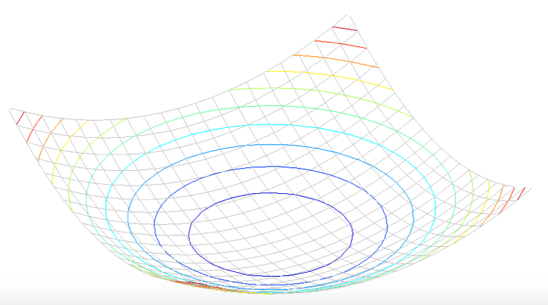
fig = plt.figure()
#ax = fig.gca(projection='3d')
ax = plt.axes(projection='3d')
X = np.arange(0,13)
Y = np.arange(0,13)
X, Y = np.meshgrid(X, Y)
Z = E
surf = ax.plot_surface(X, Y, Z, cmap=cm.coolwarm, linewidth=0, antialiased=False)
#ax.set_zlim(-1.01, 1.01)
#ax.zaxis.set_major_locator(LinearLocator(10))
#ax.zaxis.set_major_formatter(FormatStrFormatter('%.02f'))
# Add a color bar which maps values to colors.
fig.colorbar(surf, shrink=0.5, aspect=5)
plt.show()

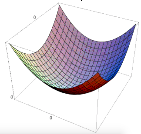
Analyzing E(u,v)
The shape of $E(u,v)$ tells us about the underlying image structure: flat region, edge region, or corner region. Lets try to figure out how $E(u,v)$ behaves for small shifts $(u,v)$. We can use Taylor Series to approximate $E$ around $(u,v)$.
$$ E(u,v) = E(0,0) + \left[ \begin{array}{cc} u & v \end{array} \right] \left[ \begin{array}{c} E_u(0,0) \\ E_v(0,0) \end{array} \right] + \frac{1}{2} \left[ \begin{array}{cc} u & v \end{array} \right] \left[ \begin{array}{cc} E_{uu}(0,0) & E_{uv}(0,0) \\ E_{uv}(0,0) & E_{vv}(0,0) \end{array} \right] \left[ \begin{array}{c} u \\ v \end{array} \right] + \cdots $$
Lets do some maths
$$ \begin{align} E_u(u,v) & = \sum_{x,y} 2 w(x,y) \left[ I(x+u,y+v)-I(x,y) \right] I_x(x+u,y+v) \\ E_{uu}(u,v) & = \sum_{x,y} 2 w(x,y) I_x(x+u,y+v) I_x(x+u,y+v) + \sum_{x,y} 2 w(x,y) \left[ I(x+u,y+v)-I(x,y) \right] I_{xx}(x+u,y+v) \\ E_{uv}(u,v) & = \sum_{x,y} 2 w(x,y) I_y(x+u,y+v) I_x(x+u,y+v) + \sum_{x,y} 2 w(x,y) \left[ I(x+u,y+v)-I(x,y) \right] I_{xy}(x+u,y+v) \end{align} $$
Re-write Taylor Series equation using the following quantities
$$ \begin{align} E(0,0) & = 0 \\ E_u(0,0) & = 0 \\ E_v(0,0) & = 0 \\ E_{uu}(0,0) & = \sum_{x,y} 2 w(x,y) I_x(x,y) I_x(x,y) \\ E_{vv}(0,0) & = \sum_{x,y} 2 w(x,y) I_y(x,y) I_y(x,y) \\ E_{uv}(0,0) & = \sum_{x,y} 2 w(x,y) I_x(x,y) I_y(x,y) \end{align} $$
We get
$$ \begin{align} E(u,v) & \approx \frac{1}{2} \left[ \begin{array}{cc} u & v \end{array} \right] \left[ \begin{array}{cc} \sum_{x,y} 2 w(x,y) I_x(x,y) I_x(x,y) & \sum_{x,y} 2 w(x,y) I_x(x,y) I_y(x,y) \\ \sum_{x,y} 2 w(x,y) I_x(x,y) I_y(x,y) & \sum_{x,y} 2 w(x,y) I_y(x,y) I_y(x,y) \end{array} \right] \left[ \begin{array}{c} u \\ v \end{array} \right] \\ & = \sum_{x,y} w(x,y) \left[ \begin{array}{cc} u & v \end{array} \right] \left[ \begin{array}{cc} I_x^2 & I_x I_y \\ I_x I_y & I_y^2 \end{array} \right] \left[ \begin{array}{c} u \\ v \end{array} \right] \end{align} $$
With this exercise, we get the second moment matrix
$$ M = \sum_{x,y} w(x,y) \left[ \begin{array}{cc} I_x^2 & I_x I_y \\ I_x I_y & I_y^2 \end{array} \right] $$
which captures the local changes in the image around location $(x,y)$. We can use $M$ to identify if $(x,y)$ is sitting on a corner. Note also that matrix $M$ can be computed from image derivatives.
Local surface approximation
The surface $E(u,v)$ is locally approximated by a quadratic form.
$$ E(u,v) \approx \left[ \begin{array}{cc} u & v \end{array} \right] M \left[ \begin{array}{c} u \\ v \end{array} \right] $$
where
$$ M = \sum_{x,y} w(x,y) \left[ \begin{array}{cc} I_x^2 & I_x I_y \\ I_x I_y & I_y^2 \end{array} \right] $$
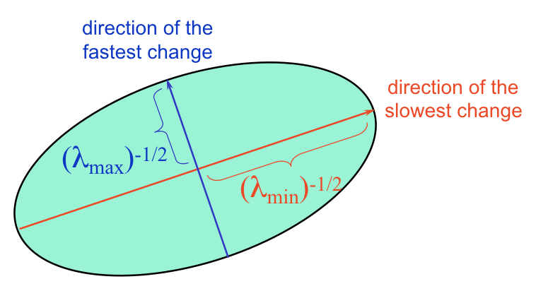
Second Moment Matrix Interpretation
Lets first consider the axis aligned case where
$$ M = \left[ \begin{array}{cc} \lambda_1 & 0 \\ 0 & \lambda_2 \end{array} \right] $$
If both $\lambda_1$ and $\lambda_2$ are close to zero, it means that there is no change along either directions (i.e., flat region). If either $\lambda_1$ or $\lambda_2$ are zero then it means that the change is only along one direction (i.e., edge region). If neither $\lambda_1$ or $\lambda_2$ are zero, it means that there is change in both directions (i.e., corner region).
We use this intuition and diagonalize matrix
$$ M = \sum_{x,y} w(x,y) \left[ \begin{array}{cc} I_x^2 & I_x I_y \\ I_x I_y & I_y^2 \end{array} \right] $$
This is accomplished by computing its eigenvectors and eigenvalues. Here eigenvectors represent the two directions, and eigenvalues represent change along these directions.
Classifying Image Pixels
Pixel is sitting in a flat region: $\lambda_1$ and $\lambda_2$ are small. $E$ is almost constant in all directions.
Pixel is sitting on an edge: $\lambda_1 \gg \lambda_2$ or $\lambda_2 \gg \lambda_1$. $E$ remains almost constant in one direction.
Pixel is sitting on a corner: $\lambda_1$ and $\lambda_2$ are large. $\lambda_1 \backsim \lambda_2$. $E$ increases in all directions.
The following corner response function formalizes these notions.
$$ \begin{align} R & = \mathrm{det}(M) - \alpha\ \mathrm{trace}(M)^2 \\ & = \lambda_1 \lambda_2 - \alpha (\lambda_1 + \lambda_2)^2 \end{align} $$
Here $\alpha$ is a constant. Typical values for $\alpha$ varies between $0.4$ and $0.6$.
Exercise
Consider the following code, that generates a 16-by-16 image. Compute 2-by-2 second moment matrix for location $(7,7)$, which is indicated as the red dot on the figure below. For this discussion, we assume that we use a window of size 5-by-5.
import cv2 as cv
import numpy as np
import matplotlib.pyplot as plt

I = np.ones((16,16), dtype='float')
I[:8,:8] = np.zeros((8,8))
plt.imshow(I, cmap='gray')
plt.plot(7,7,'ro')
plt.yticks(np.linspace(0,15,16))
plt.xticks(np.linspace(0,15,16));

# %load solutions/interest-points/solution-01.py
## Interest Points - Exercise 01

import cv2 as cv
import numpy as np
import matplotlib.pyplot as plt

I = np.ones((16,16), dtype='float')
I[:8,:8] = np.zeros((8,8))
plt.imshow(I, cmap='gray')
plt.plot(7,7,'ro')

Ix = cv.Sobel(I, cv.CV_64F, 1, 0, ksize=5)
Iy = cv.Sobel(I, cv.CV_64F, 0, 1, ksize=5)

Ix2 = np.multiply(Ix,Ix)
Iy2 = np.multiply(Iy,Iy)
IxIy = np.multiply(Ix,Iy)

SIx2 = cv.blur(Ix2, (5,5)).flatten()
SIy2 = cv.blur(Iy2, (5,5)).flatten()
SIxIy = cv.blur(IxIy, (5,5)).flatten()

M = np.vstack((SIx2, SIxIy, SIxIy, SIy2 )).reshape(4,16,16)
print('M at (7,7) =\n', M[:,7,7].reshape(2,2))
M at (7,7) =
 [[502.4  163.84]
 [163.84 502.4 ]]

Harris Corner Detector
[Harris and Stephens, 1988]
- Compute $M$ matrix for each image window to get their cornerness scores.
- Find points whose surrounding window gave large corner response.
- Take the points of local maxima, i.e., perform non-maximum suppression.

Properties
Invariance and Covariance
We want corner locations to be invariant to photometric transformations and covariant to geometric transformations
Invariance: image is transformed and corner locations do not change
Covariance: if we have two transformed versions of the same image, features should be detected in corresponding locations
Affine Intensity Change
- Corner response is partially invariant to affine intensity change
Say $I$ and $I_\mathrm{new}$ is the current and "new" instensity of a pixel then
$$ I_\mathrm{new} = a I + b $$
Notice that corner response function uses derivatives only. This suggests that it is "invariant" to change from $I$ to $I_\mathrm{new}$. However, in order to find corner locations, we need to threshold on corner response. This suggests corner response is not invariant to changes in intensity.
Specifically, corner response is invariant to intensity shift $I \to I + b$; however, corner response is not invariant to intensity scaling $I \to aI$.
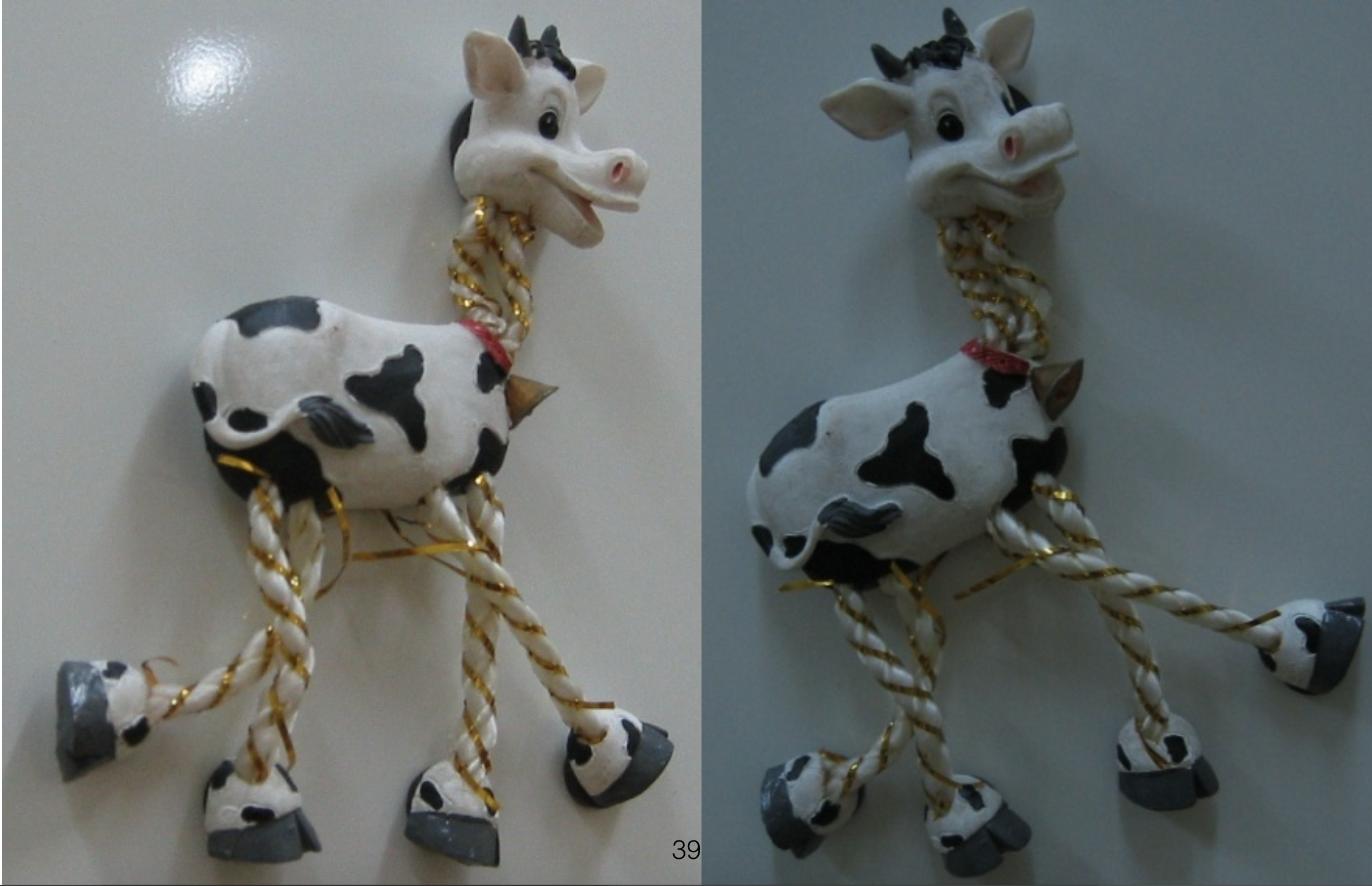
Image translation and rotation
- Corner location is covariant with respect to translation. Derivatives and window function are shift-invariant.
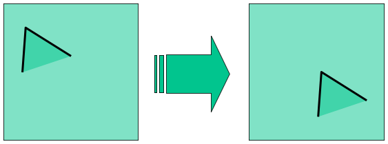
- Corner location is convariant with respect to rotation. Second moment ellipse rotates, but its shape (i.e., eigenvalues) remains the same.
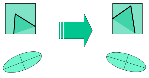
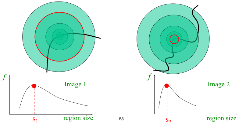
Image scaling
- Corner location is not covariant to scaling
Use multi-scale analysis for automatic scale selection for corner detection
OpenCV Harris Corner Detection
OpenCV includes a cornerHarris method to find corners in an image. We will use this built-in method to confirm our understanding of the limits of corner detection:
- covariance to translation and rotation;
- partial invariance to shifts in intensity; and
- the need for multiscale analysis to achieve scale invariance.
filename = 'data/corners-multiscale.png'
img = cv.imread(filename)
img = cv.resize(img, (256,256))
img = cv.cvtColor(img, cv.COLOR_BGR2RGB)
gray = cv.cvtColor(img, cv.COLOR_BGR2GRAY)
gray = np.float32(gray)

plt.figure(figsize=(5,5))
plt.imshow(img);

level = 0
dst = cv.cornerHarris(gray, 2, 3, 0.04)
dst = cv.dilate(dst, None)
plt.figure(figsize=(10,5))
plt.suptitle('Level = {}'.format(level))
plt.subplot(121)
plt.title('Image')
plt.xticks([])
plt.yticks([])
plt.imshow(gray, cmap='gray')
plt.subplot(122)
plt.title('Harris corner response')
plt.imshow(dst, cmap='gray')
plt.xticks([])
plt.yticks([])
([], [])

Notice that corners for three smaller squares are detected. Notice also that corner detection is covariant with respect to translation and rotation. Corner response varies with changes in intensity; however, it is somewhat robust to changes in intensity.
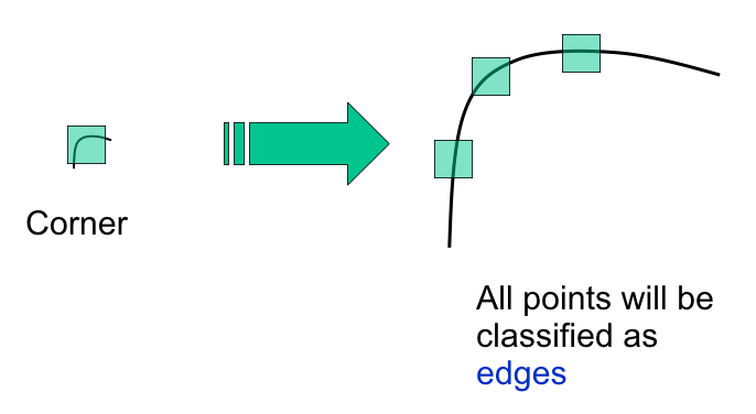
Note also that cornerHarris method is unable to find corners of rounded rectangles. At this scale these corners appear as edges.
Multiscale analysis for corner detection
We need multiscale analysis to also pick corners of the rounded rectangles.
gray_ = np.copy(gray)
level = 0
for i in range(6):
    level = level + 1
    gray_ = cv.pyrDown(gray_)
    dst = cv.cornerHarris(gray_, 2, 3, 0.04)
    dst = cv.dilate(dst, None)
    plt.figure(figsize=(10,5))
    plt.suptitle('Level = {}'.format(level))
    plt.subplot(121)
    plt.title('Image')
    plt.xticks([])
    plt.yticks([])
    plt.imshow(gray_, cmap='gray')
    plt.subplot(122)
    plt.title('Harris corner response')
    plt.imshow(dst, cmap='gray')
    plt.xticks([])
    plt.yticks([])
    plt.show()


Corner detection implementation
Below I include an implementation of corner detection that follows the "mathematical" steps that we have discussed above.
Step 1 - Load image
img_bgr = cv.imread('data/corner-test.jpg')
img = cv.cvtColor(img_bgr, cv.COLOR_BGR2RGB)
plt.figure(figsize=(7,7))
plt.imshow(img);

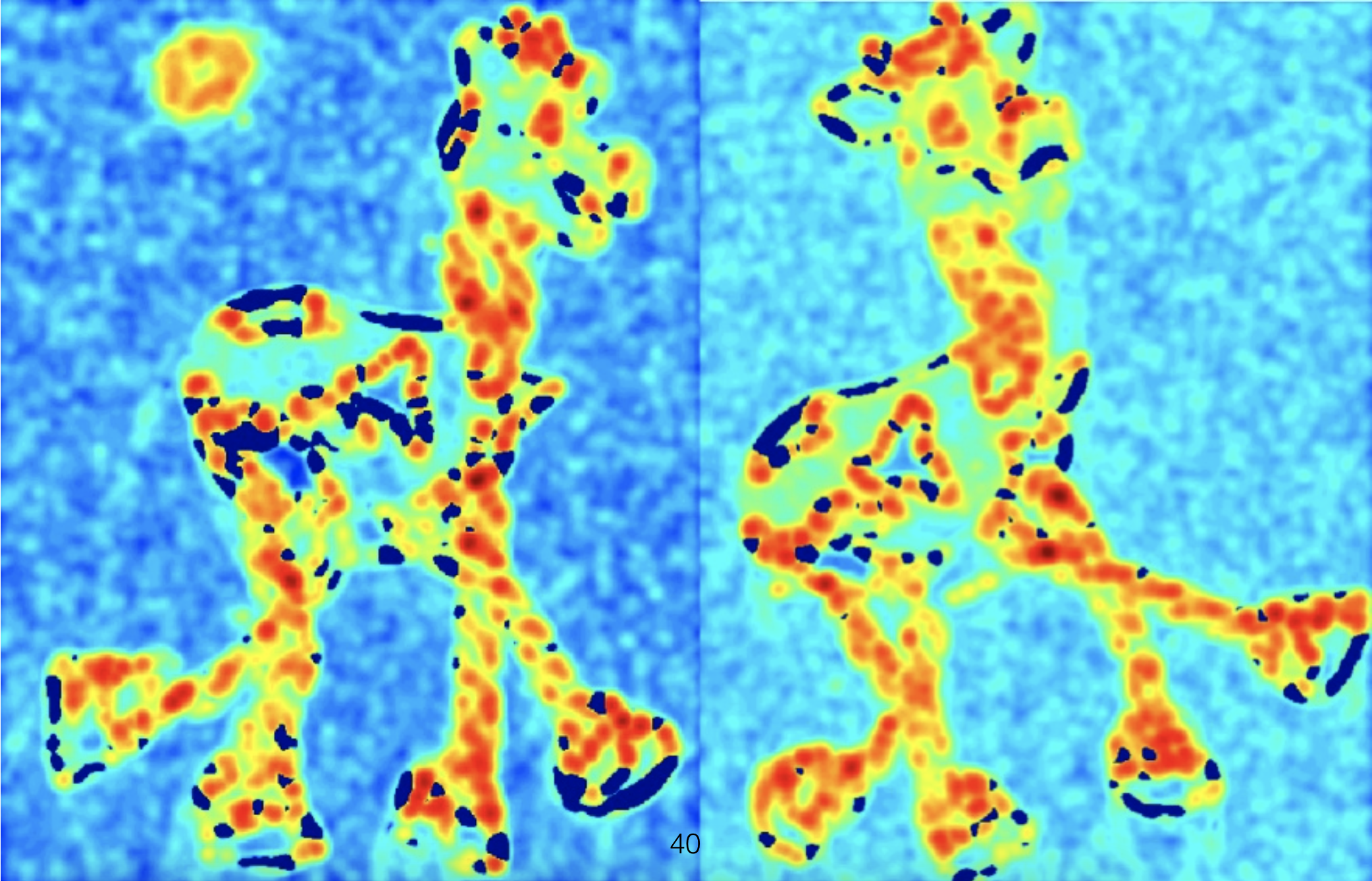
Step 2 - Compute image derivatives
Compute $I_x$ and $I_y$
img_gray = cv.cvtColor(img, cv.COLOR_RGB2GRAY)
Ix = cv.Sobel(img_gray, cv.CV_64F, 1, 0, ksize=5)
Iy = cv.Sobel(img_gray, cv.CV_64F, 0, 1, ksize=5)

plt.figure(figsize=(10,10))
plt.subplot(1,2,1)
plt.title('Ix')
plt.imshow(Ix, cmap='gray')
plt.subplot(1,2,2)
plt.title('Iy')
plt.imshow(Iy, cmap='gray');

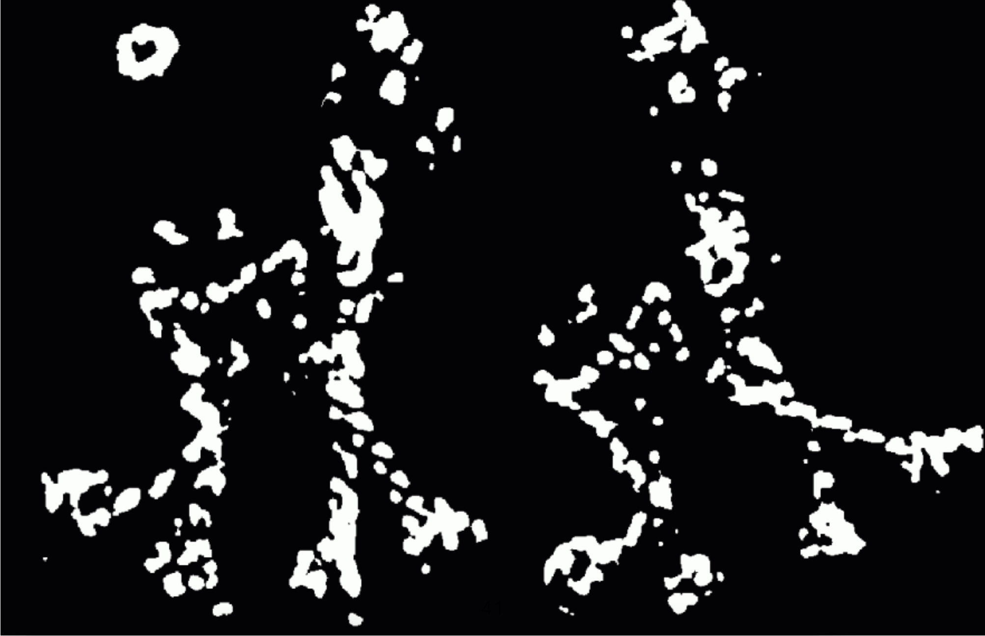
Step 3 - 2-by-2 moment matrix
Compute $I_x^2$, $I_y^2$, and $I_x I_y$ that are needed for the $2$-by-$2$ moment matrices. We choose 5-by-5 neighbourhood around each pixel to compute its moment matrix.
Ix2 = np.multiply(Ix,Ix)
Iy2 = np.multiply(Iy,Iy)
IxIy = np.multiply(Ix,Iy)

plt.figure(figsize=(20,20))
plt.subplot(1,3,1)
plt.title(r'$I_x^2$')
plt.imshow(Ix2, cmap='gray')
plt.subplot(1,3,2)
plt.title(r'$I_y^2$')
plt.imshow(Iy2, cmap='gray')
plt.subplot(1,3,3)
plt.title(r'$I_xI_y$')
plt.imshow(IxIy, cmap='gray');

SIx2 = cv.blur(Ix2, (5,5))
SIy2 = cv.blur(Iy2, (5,5))
SIxIy = cv.blur(IxIy, (5,5))

plt.figure(figsize=(20,20))
plt.subplot(1,3,1)
plt.title(r'$\sum w I_x^2$')
plt.imshow(SIx2, cmap='gray')
plt.subplot(1,3,2)
plt.title(r'$\sum w I_y^2$')
plt.imshow(SIy2, cmap='gray')
plt.subplot(1,3,3)
plt.title(r'$\sum w I_xI_y$')
plt.imshow(SIxIy, cmap='gray');

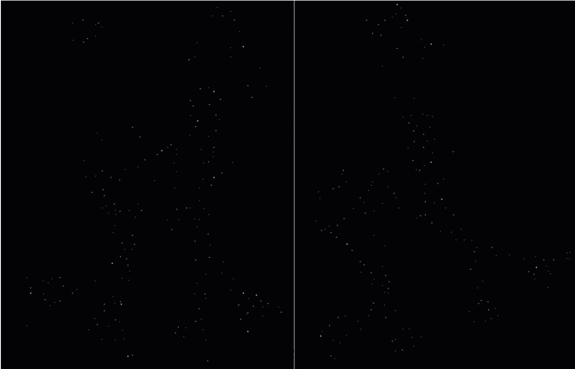
Step 4 - use momement matrix eigenvalues to compute corner response
Use eigenvalues of the moment matrix to compute corner response at each location
def find_corners(SIx2, SIy2, SIxIy):
    corners = []
    alpha = 0.04
    response = np.zeros(SIx2.shape, dtype='float32')
    for (x,y),_ in np.ndenumerate(SIx2):
        M = np.array([[SIx2[x,y], SIxIy[x,y]], [SIxIy[x,y], SIy2[x,y]]])
        w, _ = np.linalg.eig(M)
        response[x,y] = w[0]*w[1] - alpha*(w[0]+w[1])*(w[0]+w[1])
    return response

response = find_corners(SIx2, SIy2, SIxIy)
plt.figure(figsize=(10,10))
plt.imshow(response,cmap='gray');
