Frequency analysis and Fourier Transform

Faisal Qureshi
Professor
Faculty of Science
Ontario Tech University
Oshawa ON Canada
http://vclab.science.ontariotechu.ca

Copyright information

© Faisal Qureshi

License

This work is licensed under a Creative Commons Attribution-NonCommercial 4.0 International License.

Lesson Plan

• Frequency analysis of images
• Fourier transform
• Inverse Fourier transform
• Discrete Fourier transform
  • Fast Fourier transform (FFT)
• Nyquist theorem
• Convolution theorem
• Properties of Fourier transform
• Fourier transform of an Image
• Why FFT?

Periodic Functions

A function $f(t)$ is periodic of period $T$ if there is a number $T > 0$ such that $$ f(t+T) = f(t) $$ for all $t$.

Fundmental Period

The smallest $T$ for which the above relationship holds. Every integer multiple of the fundamental period is also a period: $$ f(t+nT) = f(t)\text{,\ for }n=0,\pm 1,\pm 2, \cdots. $$

Example

import numpy as np
import matplotlib.pyplot as plt
t = np.linspace(0,4*2*np.pi,100)

plt.figure(figsize=(8,2))
plt.title(f'Period = 2 $\\pi$ ({2*np.pi} in radians)')
plt.plot(t,np.cos(t),label='cos(t)')
plt.plot(t,np.sin(t),label='sin(t)')
plt.xlabel('Radians')
plt.legend()

<matplotlib.legend.Legend at 0x1050add30>

t = np.linspace(0,4,100)
plt.figure(figsize=(8,2))
plt.plot(t,np.cos(2*np.pi*t),label=f'cos(2 $\\pi$ t)')
plt.plot(t,np.sin(2*np.pi*t),label=f'sin(2 $\\pi$ t)')
plt.xlabel('Time: $t$')
plt.legend()

<matplotlib.legend.Legend at 0x10535b4d0>

t = np.linspace(0,4,512)
plt.figure(figsize=(8,4))
plt.plot(t,np.cos(2*np.pi*t),label='$\\cos 2 \\pi t$')
plt.title(f'$\\cos 2 \\pi t$')
plt.legend()
plt.xlabel('Time: $t$')

Text(0.5, 0, 'Time: $t$')

t = np.linspace(0,4,512)
plt.figure(figsize=(8,4))
plt.ylim([-1, 1])
plt.plot(t,0.5*np.cos(4*np.pi*t), label='$0.5 \\cos 4 \\pi t$')
plt.title(f'$0.5 \\cos 4 \\pi t$')
plt.legend()
plt.xlabel('Time: $t$')

Text(0.5, 0, 'Time: $t$')

t = np.linspace(0,4,512)
plt.figure(figsize=(8,4))
plt.plot(t,np.cos(2*np.pi*t) + 0.5*np.cos(4*np.pi*t), label = 'sum')
plt.title(f'$\\cos 2 \\pi t + 0.5 \\cos 4 \\pi t$')
plt.legend()
plt.xlabel('Time: $t$')

Text(0.5, 0, 'Time: $t$')

Q. What is the period of $\cos 2 \pi t$?

Answer: 1

\begin{eqnarray} \cos 2 \pi (t + 1) &=& \cos ( 2 \pi t + 2 \pi) \\ &=& \cos 2 \pi t \end{eqnarray}

Q. What is the period of $\cos 4 \pi t$?

Answer: $\frac{1}{2}$

\begin{eqnarray} \cos 4 \pi \left(t + \frac{1}{2} \right) &=& \cos \left( 4 \pi t + 4 \pi \frac{1}{2} \right) \\ &=& \cos ( 4 \pi t + 2 \pi) \\ &=& \cos ( 4 \pi t) \end{eqnarray}

Q. What is the period of $\cos 2 \pi t + \frac{1}{2} \cos 4 \pi t?$

Answer: 1 (Can you show it?)

$$ \begin{eqnarray} \cos 2 \pi (t + 1) + \frac{1}{2} \cos 4 \pi (t+1) &=& \cos (2 \pi t + 2 \pi) + \frac{1}{2} \cos (4 \pi t + 4 \pi) \\ &=& \cos 2 \pi t + \frac{1}{2} \cos (4 \pi t + (2)2 \pi) \\ &=& \cos 2 \pi t + \frac{1}{2} \cos 4 \pi t \\ \end{eqnarray} $$

Q. Is the sum of two periodic functions a periodic function?

Answer: The answer to this question is a No if you are mathematician, and it is a Yes if you are an engineer. Why no? In part due to irrational numbers. E.g., $\sqrt{2}$. Recall that irrational numbers cannot be expressed as a ratio of two integers and their decimals places go on for ever without repeating, i.e., non-terminating and non-repeating. $pi$ is another example of an irrational number.

Harmonic Oscillator

A classic example of temporal periodicity. E.g., a mass-spring system without friction. The state of this system is descrbied by $$ \begin{eqnarray} A \sin (\omega t + \phi) &=& A \sin ( 2 \pi f t + \phi ). \end{eqnarray} $$ Here, $A$ refers to amplitude, $\phi$ refers to phase, $w$ refers to the angular frequency, and $f$ refers to frequency. The two are related as $\omega = 2 \pi f$.

Exercise: show that the period of $ A \sin ( 2 \pi f t + \phi ) $ is $\frac{1}{f}$.

\begin{eqnarray} A \sin \left( 2 \pi f \left(t + \frac{1}{f} \right) + \phi \right) &=& A \sin \left( 2 \pi f t + 2 \pi f \left( \frac{1}{f} \right) + \phi \right) \\ &=& A \sin ( 2 \pi f t + 2 \pi + \phi ) \\ &=& A \sin ( 2 \pi f t + \phi ) \end{eqnarray}

Towards sum of sinusoids.

The classic example of spatial periodicity, the example that started the whole subject, is the distribution of heat in a circular ring. A ring is heated up, somehow, and the heat then distributes itself, somehow, through the material. In the long run we expect all points on the ring to be of the same temperature, but they won’t be in the short run. At each fixed time, how does the temperature vary around the ring?

Taken from Lecture Notes for Stanford EE 261 by Prof. B. Osgood

Ring can be modeled as a circle and the coordinate description of the ring where each position can be represented by an angle enforces periodicity. Recall that posiiton $\theta$ is the same as $\theta + 2 \pi$.

Temperature around the ring (or circle) cannot be described using a single sinosoid (as in harmonic oscillator). Fourier suggested to use a sum of sinosoids as a model for temperature distribution: $$ \sum_{n=1}^N A_n \sin (n \theta + \phi_n). $$

Aside: the individual terms in the above sum are referred to as harmonics.

Jean Baptiste Joseph Fourier (1786 — 1830)

• Any univariate function can be re-written as a sum of sines and cosines of different frequencies (1807)
• No one believed him
• Not translated into English until 1878
• It’s true, and it is called Fourier Series

Sums of sine and cosine

So, we can use sums of sinosoids to build complex functions $$ \sum_{n=1}^N A_n \sin (2 \pi n t + \phi_n). $$

It is, however, mathematically more convenient to re-write the sum as (see below for explanation) $$ \sum_{n=1}^N \left( a_n \cos (2 \pi n t) + b_n \sin (2 \pi n t ) \right). $$

We can further expand it by including the $0$ (constant) term. $$ \frac{a_0}{2} + \sum_{n=1}^N \left( a_n \cos (2 \pi n t) + b_n \sin (2 \pi n t ) \right). $$ Here we set the first coefficient equal to $\frac{a_0}{2}$ to make subsequent calculations easier.

Aside

\begin{eqnarray} A_n \sin (2 \pi n t + \phi_n) &=& A_n \left( \sin (2 \pi n t) \cos \phi + \cos (2 \pi n t) \sin \phi \right) \\ &=& a_n \cos (2 \pi n t) + b_n \sin (2 \pi n t ) \end{eqnarray} where $a_n = A_n \sin \phi$ and $b_n = A_n \cos \phi$, therefore $$ \sum_{n=1}^N A_n \sin (2 \pi n t + \phi_n) = \sum_{n=1}^N \left( a_n \cos (2 \pi n t) + b_n \sin (2 \pi n t ) \right). $$

Complex exponentials to rescue

Recall that $$ \cos t = \frac{e^{it} + e^{-it}}{2} $$ and $$ \sin t = \frac{e^{it} - e^{-it}}{2i} $$ where $i = \sqrt{-1}$.

Using this we can write $$ \cos (2 \pi n t) = \frac{e^{2 \pi i n t} + e^{-2 \pi i n t}}{2} $$ and $$ \sin (2 \pi n t) = \frac{e^{2 \pi i n t} - e^{-2 \pi i n t}}{2i} $$

Re-writing the sum of sinosoids in terms of complex exponentials

With these trigonometric expressions, we get

\begin{eqnarray} a_n \cos (2 \pi n t) + b_n \sin (2 \pi n t ) &=& a_n \frac{e^{2 \pi i n t} + e^{-2 \pi i n t}}{2} + b_n \frac{e^{2 \pi i n t} - e^{-2 \pi i n t}}{2i} \\ &=& \frac{ i a_n ( e^{2 \pi i n t} + e^{-2 \pi i n t} ) + b_n ( e^{2 \pi i n t} - e^{-2 \pi i n t} ) }{2i} \\ &=& \frac{ i a_n ( e^{2 \pi i n t} + e^{-2 \pi i n t} ) + b_n ( e^{2 \pi i n t} - e^{-2 \pi i n t} ) }{2i} \times \frac{i}{i} \\ &=& \frac{ (-1) a_n ( e^{2 \pi i n t} + e^{-2 \pi i n t} ) + i b_n ( e^{2 \pi i n t} - e^{-2 \pi i n t} ) }{2(-1)} \\ &=& \frac{ a_n ( e^{2 \pi i n t} + e^{-2 \pi i n t} ) - i b_n ( e^{2 \pi i n t} - e^{-2 \pi i n t} ) }{2} \\ &=& \frac{ a_n e^{2 \pi i n t} + a_n e^{-2 \pi i n t} - i b_n e^{2 \pi i n t} + i b_n e^{-2 \pi i n t} ) }{2} \\ &=& \frac{a_n - ib_n}{2} e^{2 \pi i n t} + \frac{a_n + ib_n}{2} e^{- 2 \pi i n t} \end{eqnarray}

Expanding further

\begin{eqnarray} \frac{a_0}{2} + \sum_{n=1}^N \left( a_n \cos (2 \pi n t) + b_n \sin (2 \pi n t ) \right) &=& \frac{a_0}{2} + \sum_{n=1}^N c_n e^{2 \pi n t} + \sum_{n=-N}^{-1} c_{n} e^{2 \pi n t} \\ &=& \sum_{n=-N}^N c_n e^{2 \pi i nt}. \end{eqnarray} Here $c_0 = \frac{a_0}{2}$, $c_n = \frac{a_n - ib_n}{2}$, and $c_{-n} = \frac{a_n + ib_n}{2}$.

Coefficients $c_n$ are complex numbers that satisfy $$ c_{-n} = \overline {c_n}. $$ Also $$ c_{0} = \overline {c_0}; $$ therefore, $c_{0}$ is a real-number.

A little detour about complex numbers

The conjugate of a complex number $$ c = a + b i $$ is $$ \overline{c} = a - b i $$

Is this sum real?

Say we have a complex looking 1D periodic signal $f(t)$. Lets scale this signal such that its period is $1$.

Let's consider the terms containing $c_n$ and its conjugate $\overline{c_n}$. We get

\begin{eqnarray} c_n e ^ {2 \pi i n t} + c_{-n} e ^ {- 2 \pi i n t} &=& c_n e ^ {2 \pi i n t} + \overline{c_{n}} \overline{e ^ {2 \pi i n t}} \\ &=& 2 \text{Re} (c_n e^{2 \pi i n t}) \end{eqnarray}

Therefore,

\begin{eqnarray} \sum_{n=-N}^{N} c_n e ^ {2 \pi i n t} &=& \sum_{n=0}^{N} 2 \text{Re}(c_n e ^ {2 \pi i n t}) \\ &=& 2 \text{Re} \{ \sum_{n=0}^N e^{2 \pi i n t} \}, \end{eqnarray}

This shows that the sum is a real number.

Solving for $c_n$s

Say we have a periodic function $f(t)$. Furthermore, assume that we have scaled $t$ such that the function has a period of $1$ (it repeats itself after every $1$ second, for example).

$$ f(t) = \sum_{n=-N}^N c_n e^{2 \pi i n t}. $$

How do we solve for $c_n$? Note that all other items on the R.H.S. are known.

Beginning

Let's try to solve it for a particular $c_k$. If we can solve it for a particular $k \in [-N,N]$ then we can compute $c_n$s.

Step 1: Multiply both sides by $e^{- 2 \pi i k t}$ to isolate $c_k$.

$$ \begin{eqnarray} e^{- 2 \pi i k t} f(t) &=& e^{- 2 \pi i k t} \sum_{n=-N}^N c_n e^{2 \pi i n t} \\ &=& \cdots + e^{- 2 \pi i k t} c_k e^{2 \pi i k t} + \cdots \\ &=& \cdots + c_k + \cdots \end{eqnarray} $$

Moving things around we get

$$ \begin{eqnarray} c_k &=& e^{- 2 \pi i k t} f(t) - \sum_{n=-N,n \neq k}^{N} c_n e^{-2 \pi i k t} e^{-2 \pi i n t} \\ &=& e^{- 2 \pi i k t} f(t) - \sum_{n=-N,n \neq k}^{N} c_n e^{2 \pi i (n - k) t} \end{eqnarray} $$

Ok, so we have been able to isolate $c_k$ on the L.H.S.; however, we are not done yet. The terms on the R.H.S. include $c_n$ where $n \neq k$. We need to do something more.

Step 2: Integrate both sides between $0$ and $1$. Recall that we assumed that $f(t)$ has a period of $1$. Any intervals of length $1$ should work due to periodicity.

$$ \begin{eqnarray} \int_0^1 c_k dt &=& \int_0^1 \left( e^{- 2 \pi i k t} f(t) - \sum_{n=-N,n \neq k}^{N} c_n e^{2 \pi i (n - k) t} \right) dt \\ \left[c_k t \right]_0^1 &=& \int_0^1 e^{- 2 \pi i k t} f(t) dt - \int_0^1 \sum_{n=-N,n \neq k}^{N} c_n e^{2 \pi i (n - k) t} dt \\ c_k (1-0) &=& \int_0^1 e^{- 2 \pi i k t} f(t) dt - \sum_{n=-N,n \neq k}^{N} c_n \int_0^1 e^{2 \pi i (n - k) t} dt \\ c_k &=& \int_0^1 e^{- 2 \pi i k t} f(t) dt - \sum_{n=-N,n \neq k}^{N} c_n \int_0^1 e^{2 \pi i (n - k) t} dt \end{eqnarray} $$

Using the property that integral of the sum is the sum of integrals to re-write the R.H.S. above.

Consider for $n \neq k$ $$ \begin{eqnarray} \int_0^1 e^{2 \pi i (n - k) t} dt &=& \left[ \frac{1}{2 \pi i (n-k)} e ^{2 \pi i (n-k) t} \right]_{t=0}^{t=1} \\ &=& \frac{1}{2 \pi i (n-k)} ( e ^{2 \pi i (n-k) } - e^0) \\ &=& \frac{1}{2 \pi i (n-k)} ( 1 - 1) \\ &=& 0 \end{eqnarray} $$

This suggets

$$ \begin{eqnarray} c_k &=& \int_0^1 e^{- 2 \pi i k t} f(t) dt. \end{eqnarray} $$

We are able to compute $c_k$s given a function $f(t)$!

Aside: Showing $e ^{2 \pi i (n-k) } = 1$

Recall that $$ e^{it} = \cos t + i \sin t $$ and $$ e^{-it} = \cos t - i \sin t $$

Using these we get

$$ \begin{eqnarray} e ^{2 \pi i (n-k) } &=& \cos (2 \pi (n-k)) + i \sin (2 \pi (n-k)) \\ &=& \cos (0 + (n-k) 2 \pi ) + i \sin ( 0 + (n-k) 2 \pi) \\ &=& \cos (0) + \sin(0) \\ &=& 1 + 0 \\ &=& 1 \end{eqnarray} $$

Afterword

We just showed that if we can write a periodic function $f(t)$ with a period of $1$ as the sum

$$ f(t) = \sum_{n=-N}^{N} c_n e^{2 \pi i n t} $$

then the coefficients $c_n$ are computed as

$$ c_n = \int_{0}^{1} e^{-2 \pi i n t} f(t) dt $$

Be wary that we have not yet shown that every periodic function can be expressed as the sum of complex exponentials.

A point about real signals

In our calculations for arriving at $c_n$ we have not assumed a real signal. Assuming $f(t)$ is a real signal let's find the relationship between $\overline{c_n}$ and $c_{-n}$.

$$ \begin{eqnarray} \overline{c_n} &=& \overline { \int_{0}^{1} e^{-2 \pi i n t} f(t) dt } \\ &=& \int_{0}^{1} \overline{ e^{-2 \pi i n t}} \overline{f(t)} dt \\ &=& \int_{0}^{1} \overline{ e^{-2 \pi i n t}} \ \overline{f(t)} dt \\ &=& \int_{0}^{1} e^{2 \pi i n t} f(t) dt \text{\ \ \ (because\ } f(t) \text{\ and\ } t \text{\ and\ } dt \text{\ are real)}\\ &=& \int_{0}^{1} e^{- 2 \pi i (-n) t} f(t) dt \\ &=& c_{-n} \end{eqnarray} $$

Fourier Series

Sum $$ f(t) = \sum_{n=-N}^{N} c_n e^{2 \pi i n t} $$ is called a (Finite) Fourier series.

Fourier Coefficients

Coefficients $$ c_n = \int_{0}^{1} e^{-2 \pi i n t} f(t) dt $$ are referred to as Fourier coefficients.

A commonly used notation for Fourier Coefficients

Often times we use the following notation instead to denote Fourier coefficients

$$ \hat{f}(n) = \int_{0}^{1} e^{-2 \pi i n t} f(t) dt $$

The following also works (since the integral is computed over an interval of length $1$, and we have already assumed that function $f(t)$ is of period $1$.)

$$ \hat{f}(n) = \int_{-\frac{1}{2}}^{\frac{1}{2}} e^{-2 \pi i n t} f(t) dt $$

This also means we can re-write the Fourier series as

$$ f(t) = \sum_{n=-N}^{N} \hat{f}(n) e^{2 \pi i n t} $$

Frequency vs. Harmonics

Frequency in Fourier Series

• Frequency refers to how many cycles a wave completes per unit of time.
• In the Fourier series, the term $e^{2\pi i n t}$ represents oscillations at a frequency proportional to $n$, where $n$ is an integer.
• The fundamental frequency $f_0$ corresponds to $n = 1$. Higher frequencies are multiples of this fundamental frequency.

Harmonics in Fourier Series

• Harmonics are integer multiples of the fundamental frequency.
  • The 1st harmonic corresponds to the fundamental frequency ($n = 1$).
  • The 2nd harmonic corresponds to $2f_0$ ($n = 2$).
  • The 3rd harmonic corresponds to $3f_0$ ($n = 3$), and so on.
• In the Fourier series, each term $n$ represents a harmonic: $$ \hat{f}(n) e^{2\pi i n t} $$ where $n = 1, 2, 3, \dots $ are the harmonics, and $\hat{f}(n)$ is the coefficient representing its amplitude and phase.

Key Difference

• Frequency: Refers to the rate of oscillation (e.g., cycles per second).
• Harmonics: Specific frequencies that are integer multiples of the fundamental frequency. They are discrete components of the overall waveform.

Example

For a function $f(t)$ with a fundamental frequency of $f_0 = 1 \, \text{Hz}$:

• The 1st harmonic has a frequency of $1 \, \text{Hz}$.
• The 2nd harmonic has a frequency of $2 \, \text{Hz}$.
• The 3rd harmonic has a frequency of $3 \, \text{Hz}$, and so on.

Each harmonic contributes to the overall shape of the periodic waveform.

What does this all mean?

The ability to write $f(t)$ as a Fourier series means that the function $f(t)$ is formed of many harmonics (alternately, many frequencies), both negative and positive, may be an infinite number of these.

The set of frequencies present in a given periodic signal is spectrum of the signal.

Keep in mind that frequencies make up the spectrum, and not their coefficients.

It is possible to have some coefficients zero. It is also possible that $\hat{f}{n} = 0$ for $|n| > N$. Then we say that the signal is bandlimited with a $bandwidth=N$.

It is possible to construct a power spectrum (or energy spectrum) of a signal by ploting the square magnitudes $|\hat{f}(n)|^2$.

Dealing with functions with period other then $1$

Notation alert. I am again using $c_n$ instead of $\hat{f}(n)$ in the following section.

Say we have a function $f(t)$ with period $T$. This means that $f(t+T) = f(t)$.

Let's define a function $$ g(t) = f(Tt). $$ The period of function $g(t)$ is $1$ since $$ \begin{eqnarray} g(t + 1) &=& f(T(t+1)) \\ &=& f(Tt + T) \\ &=& f(Tt) \text{\ (Because $f(t)$ has a period of $T$} )\\ &=& g(t) \end{eqnarray} $$

Expressing functions of period $T$ as sum of harmonics.

Let's write out the finite Fourier series $$ g(t) = \sum_{n=-N}^N c_n e^{2 \pi i n t} $$ Now set $s = Tt$ then $g(t) = f(s)$. Rewrite the sum $$ \begin{eqnarray} f(s) &=& g(t) \\ &=& \sum_{n=-N}^N c_n e^{2 \pi i n t} \\ &=& \sum_{n=-N}^N c_n e^{2 \pi i n s/T} \end{eqnarray} $$

This means that we are indeed able to express periodic functions of period $T$ as sums of harmonics $e^{2 \pi i n s/T}$. Similarly, we can also re-write the expression for computing $c_n$ using the same change of variables.

Computing $c_n$s for functions $f(t)$ of period $T$

We have

$$ f(t) = \sum_{n=-N}^N c_n e^{2 \pi i n t/T} $$

Step 1: Multiply both sides by $e^{- 2 \pi i k t/T}$

$$ \begin{eqnarray} e^{- 2 \pi i k t/T} f(t) &=& e^{- 2 \pi i k t/T} \sum_{n=-N}^N c_n e^{2 \pi i n t/T} \\ &=& \cdots + e^{- 2 \pi i k t/T} c_k e^{2 \pi i k t/T} + \cdots \\ &=& \cdots + c_k + \cdots \end{eqnarray} $$

Moving things around we get

$$ \begin{eqnarray} c_k &=& e^{- 2 \pi i k t/T} f(t) - \sum_{n=-N,n \neq k}^{N} c_n e^{-2 \pi i k t/T} e^{-2 \pi i n t/T} \\ &=& e^{- 2 \pi i k t/T} f(t) - \sum_{n=-N,n \neq k}^{N} c_n e^{2 \pi i (n - k) t/T} \end{eqnarray} $$

Step 2: Integrate over period $T$

$$ \begin{eqnarray} \int_{0}^T c_k dt &=& \int_{0}^T \left( e^{- 2 \pi i k t/T} f(t) - \sum_{n=-N,n \neq k}^{N} c_n e^{2 \pi i (n - k) t/T} \right) dt \\ c_k T &=& \int_{0}^T e^{- 2 \pi i k t/T} f(t) dt - \sum_{n=-N,n \neq k}^{N} \int_0^T c_n e^{2 \pi i (n - k) t/T} dt \\ c_k &=& \frac{1}{T} \int_{0}^T e^{- 2 \pi i k t/T} f(t) dt \end{eqnarray} $$

The second term on the R.H.S. is equal to zero following similar reasoning as we did for functions of period $1$.

Putting it together

For functions $f(t)$ of period $T$, we get the following expressions

$$ \begin{eqnarray} f(t) &=& \sum_{n=-N}^{N} \hat{f}(n) e^{2 \pi i n t/T} \\ \hat{f}(n) &=& \frac{1}{T} \int_{-\frac{T}{2}}^{\frac{T}{2}} e^{-2 \pi i n t/T} f(t) dt \end{eqnarray} $$

We can go back and forth between $\hat{f}(n)$ from $f(t)$.

Phase, Amplitude, and Frequency

Given $\hat{f}(n)$, we can compute the amplitude, phase and frequency as follows.

Recall that $\hat{f}(n) = a_n + i b_n $ then

Phase $$\phi_n = \arctan \left( \frac{b_n}{a_n} \right).$$

Amplitude $$A_n = \pm \sqrt{a^2 + b^2}$$

Frequency $$f_n = \frac{n}{T} $$

Relationship between time domain and frequency domain

Fourier series captures the relationship between time (say, it can be spatial domain) domain $f(t)$ and frequency domain $\hat{f}(n)$. In the time domain the signal repeats itself after $T$ (say, seconds), where as the spectrum contains points $0, \pm 1/T, \pm 2/T, \cdots$. Note that these points sit $1/T$ apart.

The larger the period in time the smaller the spacing of the spectrum. The smaller the period in time, the larger the spacing of the spectrum.

Taken from Lecture Notes for Stanford EE 261 by Prof. B. Osgood

Fourier Transform and Inverse Fourier Transform

Fourier Transform

Fourier transform of function $f(t)$ of period $T$ involves computing $\hat{f}(n)$ (or co-efficients of the Fourier series). This is accomplished using $$ \hat{f}(n) = \frac{1}{T} \int_{-\frac{T}{2}}^{\frac{T}{2}} e^{-2 \pi i n t/T} f(t) dt $$

We often denote this proces as $$ \hat{f}(n) = \mathcal{F}\{ f(t) \} $$

Inverse Fourier Transform

Inverse Fourier transform recovers the original signal $f(t)$ from its Fourier series $\hat{f}(n)$. This is accomplished using

$$ f(t) = \sum_{n=-N}^{N} \hat{f}(n) e^{2 \pi i n t/T} $$

We usually denote inverse Fourier transform as $$ f(t) = \mathcal{F}^{-1}\{ \hat{f}(n) \} $$

Missing topics

These notes do not cover Fourier transform for continuous signals and discrete time Fourier transform. I encourage the interested reader to find a good text book on signal processing to continue their investigations into Fourier transform and its many uses.

Discrete Fourier Transform (DFT)

A sequence of $N$ numbers

$$ x_0, x_1, x_2, \cdots, x_{N-1} $$

can be transformed into an $N$-periodic sequence of complex numbers

$$ X_k = \sum_{n=0}^{N-1} x_n e^{- 2 \pi i \frac{k}{N} n} \text{, for } k=0, 1, 2, \cdots, N-1 $$

Fast Fourier Transform (FFT) is $N \log N$.

It is easy to recover the original sequence $x$ given its Fourier transform $X$ as follows:

$$ x_n = \frac{1}{N} \sum_{k=0}^{N-1} X_k e^{2 \pi i \frac{k}{N} n}. $$

Key idea: sum of sinosoids

import numpy as np
import scipy as sp
from scipy import signal
import matplotlib.pyplot as plt

Plotting sine wave

Consider a Sine Wave

$$ y = a \sin(\omega t + \phi) $$

Here $\omega$ represents angular frequency and $\phi$ represents phase. Recall that $t$ is time and $\omega = 2 \pi f$, where $f$ is frequency.

t = np.linspace(0, 1, 1000)

a = 1 # amplitude
f = 1 # frequency
p = 0 # phase
omega = 2 * np.pi * f # angular velocit
y = a * np.sin( omega * t + p)

plt.figure(figsize=(10, 4))
plt.title(f'Sine wave for amplitude={a}, $\\omega$={f}, and $\\phi$={p}')
plt.plot(t, y, 'k')
plt.xlabel('$t$')
plt.ylabel(f'$a \\sin(2 \\pi \\omega t + \\phi)$');

Sine waves with different frequencies and phases.

t = np.linspace(0, 1, 1000)

a1 = 1
f1 = 1
p1 = 0*np.pi/180.0
omega1 = 2 * np.pi * f1
y1 = a1 * np.sin( omega1 * t + p1)

a2 = 0.4
f2 = 3
p2 = 90*np.pi/180.0
omega2 = 2 * np.pi * f2
y2 = a2 * np.sin( omega2 * t + p2)

a3 = 1.7
f3 = 10
p3 = 45*np.pi/180.0
omega3 = 2 * np.pi * f3
y3 = a3 * np.sin( omega3 * t + p3)


plt.figure(figsize=(10,4))
plt.title(f'Sine wave having different frequencies and waves')
plt.plot(t, y1, 'r-.', label=f'$a$={a1} $f$={f1}, $\\phi$={p1*180./np.pi:4.3}')
plt.plot(t, y2, 'b--', label=f'$a$={a2} $f$={f2}, $\\phi$={p2*180/np.pi:4.3}')
plt.plot(t, y3, 'k', label=f'$a$={a3} $f$={f3}, $\\phi$={p3*180./np.pi:4.3}')
plt.legend()
plt.xlabel('time')
plt.ylabel(f'$\\sin(2 \\pi \\omega t + \\phi)$');

Example: Adding two sine waves

y = np.zeros([2, 1000])
t = np.linspace(0, 1, 1000)

a, f, p = 1, 1, 0
omega = 2 * np.pi * f
y[0,:] = a * np.sin( 2 * omega * t + p)

a, f, p = 1/3, 3, 0
omega = 2 * np.pi * f
y[1,:] = a * np.sin( 2 * omega * t + p)

plt.figure(figsize=(10,4))
plt.plot(t, y[0,:], 'r-.', label=f'$a$=1,  f={1}, $\\phi$={0}', alpha=0.5)
plt.plot(t, y[1,:], 'b--', label=f'$a$=1/3,  f={3}, $\\phi$={0}', alpha=0.5)
plt.plot(t, np.sum(y, 0), 'k', label='sum')
plt.legend();

Example: Square wave

We extend this idea to construct a square wave.

$$ y = \sum_{f=[1,3,5,\cdots]}^\infty \frac{1}{f} \sin(2 \pi f t) $$

This is quite impressive, given that sine waves themselves have no corners.

def square_wave(n_components, n_samples=1000):
    """
    Constructs a square wave using sine wave components.
    
    Returns time (t), generated wave (y), and individual components (c)
    """
    
    y = np.zeros([n_components, 1000])
    t = np.linspace(0, 1, 1000)

    a, f, p = 1, 1, 0
    for i in range(n_components):
        a = 1 / f
        omega = 2 * np.pi * f    
        y[i,:] = a * np.sin( omega * t + p)
        f += 2
        
    return t, np.sum(y, 0), y

n_components = 100
t, y, c = square_wave(n_components)

plt.figure(figsize=(10,4))
for i in range(np.min([100, n_components])):
    plt.plot(t, c[i,:], alpha=0.3)   
plt.plot(t, y, 'k', label='sum')
plt.legend();

Generating composite signals

Generate a sample signal with two sine waves (5Hz & 20Hz)

fs = 1000  # Sampling frequency (Hz)
N = 1024   # Number of samples
t = np.linspace(0, N/fs, N, endpoint=False)

# Create a composite signal (50Hz and 120Hz with different phases)
x = np.sin(2*np.pi*5*t) + 0.5*np.sin(2*np.pi*20*t + np.pi/4)

plt.figure(figsize=(6,3))
plt.plot(t, x)
plt.title(f'Length of signal = {len(x)}')

Text(0.5, 1.0, 'Length of signal = 1024')

Aside: Complex numbers in Numpy

Numpy supports complex numbers. Given a complex number x

• np.complex() constructs a complex number
• x.real refers to real component
• x.imag refers to imaginary component
• np.abs(x) computes magnitude (or amplitude above)
• np.angle(x) computes angle in radians (or phase above)

x = complex(1, 2)
print(f'complex number x    = {x}')
print(f'real part of x      = {x.real}')
print(f'imaginary part of x = {x.imag}')
print(f'magnitude of      x = {np.abs(x)}')
print(f'angle of x          = {np.angle(x)*180/np.pi} degrees')

complex number x    = (1+2j)
real part of x      = 1.0
imaginary part of x = 2.0
magnitude of      x = 2.23606797749979
angle of x          = 63.43494882292201 degrees

Implementation of DFT and Inverse DFT

Let's write some Python code to perform Discrete Fourier Transform (DFT) and Inverse DFT.

Below x denotes signal in time, and X denotes its Fourier transform.

DFT

def dft(x):
    """
    Compute the Discrete Fourier Transform (DFT) of a 1D signal x.
    """
    N = len(x)
    X = np.zeros(N, dtype=complex)
    
    for k in range(N):
        for n in range(N):
            X[k] += x[n] * np.exp(-2j * np.pi * k * n / N)
    
    return X

Inverse DFT

def idft(X):
    """
    Compute the Inverse Discrete Fourier Transform (IDFT).
    """
    N = len(X)
    x = np.zeros(N, dtype=complex)
    
    for n in range(N):
        for k in range(N):
            x[n] += X[k] * np.exp(2j * np.pi * k * n / N)
    
    return x / N  # Normalize by N

Frequencies

def fftfreq(N, sampling_rate):
    """
    Computes the frequency bins for the Discrete Fourier Transform (DFT).

    Parameters:
        N (int): Number of points in the DFT.
        d (float): Sampling interval b(1 / sampling rate).

    Returns:
        freqs (numpy array): Frequency bins.
    """
    d = 1. / sampling_rate
    
    # Create an array of indices
    freqs = np.zeros(N)
    half_N = (N-1) // 2 + 1  # Handles even and odd N

    # Compute positive frequencies
    freqs[:half_N] = np.arange(half_N) / (N * d)

    # Compute negative frequencies
    freqs[half_N:] = np.arange(-(N//2), 0) / (N * d)

    return freqs

Magnitudes

def compute_magnitude(X):
    """
    Computes the magnitude spectrum of a DFT result.
    
    Parameters:
        X (array): Complex-valued DFT output.
    
    Returns:
        magnitude (array): Magnitude spectrum.
    """
    return np.sqrt(X.real**2 + X.imag**2)  # Equivalent to np.abs(X)

Phases

def compute_phase(X):
    """
    Computes the phase spectrum of a DFT result.
    
    Parameters:
        X (array): Complex-valued DFT output.
    
    Returns:
        phase (array): Phase spectrum (in radians).
    """
    return np.arctan2(X.imag, X.real)  # Equivalent to np.angle(X)

Signal Analysis

We will show that it is possible to decompose a signal as a sum of sinosoidals

Signal

# Example: Generate a sample signal with two sine waves (50Hz & 120Hz)
fs = 1000  # Sampling frequency (Hz)
N = 1024   # Number of samples
t = np.linspace(0, N/fs, N, endpoint=False)

# Create a composite signal (50Hz and 120Hz with different phases)
x = np.sin(2*np.pi*5*t) + 0.5*np.sin(2*np.pi*20*t + np.pi/4)

plt.figure(figsize=(6,3))
plt.plot(t, x)
plt.title(f'Length of signal = {len(x)}')

Text(0.5, 1.0, 'Length of signal = 1024')

Perform DFT

X = dft(x)
frequencies = fftfreq(N=len(X), sampling_rate=fs)
magnitudes = compute_magnitude(X)
phases = compute_phase(X)

Reconstruct Signal

t_reconstruct = np.linspace(0, N/fs, N, endpoint=False)  # Time vector for reconstruction

plt.figure(figsize=(6,3))
k = 9 # This should be less than or equal to N//2, since we only care about real frequencies
plt.title(f'Sinosoid component = {k}')
plt.plot(t,(magnitudes[k] / (N//2)) * np.cos(2 * np.pi * frequencies[k] * t_reconstruct + phases[k]))

[<matplotlib.lines.Line2D at 0x1130274d0>]

# Reconstruct the signal using inverse Fourier synthesis
t_reconstruct = np.linspace(0, N/fs, N, endpoint=False)  # Time vector for reconstruction
reconstructed_signal = np.zeros_like(t_reconstruct)  # Initialize reconstructed signal

# Sum up sine waves using magnitude, frequency, and phase
for k in range(N//2):  # Use only positive frequencies, w hen reconstructing the real part of the signal, we use only the cosine term
    reconstructed_signal += (magnitudes[k] / (N//2)) * np.cos(2 * np.pi * frequencies[k] * t_reconstruct + phases[k])

# Plot original vs reconstructed signal
plt.figure(figsize=(10, 4))
plt.plot(t, x, label="Original Signal", linestyle='dashed', alpha=0.7)
plt.plot(t_reconstruct, reconstructed_signal, label="Reconstructed Signal", linewidth=1.2)
plt.xlabel("Time (s)")
plt.ylabel("Amplitude")
plt.title("Original vs Reconstructed Signal")
plt.legend()
plt.grid()
plt.show()

Conclusion

We just showed that we are able to decompose a signal into a cosines, shifted and having different frequencies, and that it is possible to recover the original signal from these cosines.

Numpy Fast Fourier Transform Routines

For all practical purposes, we will use Numpy built-in Fast Fourier Transform routines

Signal

# Example: Generate a sample signal with two sine waves (50Hz & 120Hz)
fs = 1000  # Sampling frequency (Hz)
N = 1024   # Number of samples
t = np.linspace(0, N/fs, N, endpoint=False)

# Create a composite signal (50Hz and 120Hz with different phases)
x = np.sin(2*np.pi*5*t) + 0.5*np.sin(2*np.pi*20*t + np.pi/4)

plt.figure(figsize=(6,3))
plt.plot(t, x)
plt.title(f'Length of signal = {len(x)}')

Text(0.5, 1.0, 'Length of signal = 1024')

FFT

# Compute FFT using Numpy built-in method
X = np.fft.fft(x)

Frequency, Magnitude and Phase

Recall that if we have $N$ samples then the largest frequency that we can represent in a signal is $\frac{N}{2}$. Recall also that the Fourier transform is reflected around $0$ and we also get negative frequencies.

# Compute magnitude and phase using NumPy built-in functions
frequencies = np.fft.fftfreq(N, 1/fs)
print(f'Max frequency = {np.max(frequencies)}')

magnitudes = np.abs(X)
phases = np.angle(X)

Max frequency = 499.0234375

Reconstruct the signal as before

t_reconstruct = np.linspace(0, N/fs, N, endpoint=False)  # Time vector for reconstruction
reconstructed_signal = np.zeros_like(t_reconstruct)  # Initialize reconstructed signal

# Sum up sine waves using magnitude, frequency, and phase
for k in range(N//2):  # Use only positive frequencies
    reconstructed_signal += (magnitudes[k] / (N//2)) * np.cos(2 * np.pi * frequencies[k] * t_reconstruct + phases[k])

# Plot original vs reconstructed signal
plt.figure(figsize=(10, 4))
plt.plot(t, x, label="Original Signal", linestyle='dashed', alpha=0.7)
plt.plot(t_reconstruct, reconstructed_signal, label="Reconstructed Signal", linewidth=1.2)
plt.xlabel("Time (s)")
plt.ylabel("Amplitude")
plt.title("Original vs Reconstructed Signal")
plt.legend()
plt.grid()
plt.show()

Identifying dominant frequencies

FFT analysis allows us to identify dominant frequencies present in the signal. Check magnitude (or amplitudes) for different frequencies, and pick frequencies that have large magnitudes.

# Identify dominant frequencies
num_peaks = 6  # Number of dominant frequencies to identify
positive_frequencies = frequencies[:N//2]  # Use only positive frequencies
positive_magnitudes = magnitudes[:N//2]  # Use only positive magnitudes

# Find indices of highest magnitudes
dominant_indices = np.argsort(positive_magnitudes)[-num_peaks:][::-1]  # Sort in descending order

# Extract dominant frequencies and their magnitudes
dominant_frequencies = positive_frequencies[dominant_indices]
dominant_magnitudes = positive_magnitudes[dominant_indices]

# Print results
print("Dominant Frequencies (Hz):", dominant_frequencies)
print("Corresponding Magnitudes:", dominant_magnitudes)

# Plot magnitude spectrum with dominant frequencies marked
plt.figure(figsize=(10, 4))
plt.plot(positive_frequencies, positive_magnitudes, label="Magnitude Spectrum")
plt.scatter(dominant_frequencies, dominant_magnitudes, color='red', label="Dominant Frequencies", zorder=3)
plt.xlabel("Frequency (Hz)")
plt.ylabel("Magnitude")
plt.title("Magnitude Spectrum with Dominant Frequencies")
plt.legend()
plt.grid()
plt.show()

Dominant Frequencies (Hz): [ 4.8828125 19.53125   20.5078125  5.859375  18.5546875  3.90625  ]
Corresponding Magnitudes: [496.80272823 173.18433372 152.864182    72.03052675  58.95824074
  51.16973856]

Power Spectrum

plt.figure(figsize=(10, 4))
plt.plot(frequencies[:N//2], magnitudes[:N//2])  # Only plot positive frequencies
plt.xlabel("Frequency (Hz)")
plt.ylabel("Magnitude")
plt.title("Magnitude Spectrum")
plt.grid()
plt.show()

Inverse DFT

# Compute the inverse FFT of the filtered spectrum to reconstruct the signal
reconstructed_signal = np.fft.ifft(X).real

plt.figure(figsize=(10, 4))
plt.plot(t, x, label="Original Signal", linestyle='dashed', alpha=0.7)
plt.plot(t_reconstruct, reconstructed_signal, label="Reconstructed Signal", linewidth=1.2)
plt.xlabel("Time (s)")
plt.ylabel("Amplitude")
plt.title("Original vs Reconstructed Signal")
plt.legend()
plt.grid()
plt.show()

Discarding frequencies to achieve compression

discard = 0.01

# Thresholding: Discard frequencies below a set threshold
threshold = np.max(magnitudes) * discard  # 10% of max magnitude
X_filtered = np.where(magnitudes > threshold, X, 0)  # Zero out low-magnitude frequencies

# Count how many frequencies were zeroed out
zeroed_out_count = np.sum(magnitudes <= threshold)
print(f"Number of frequencies zeroed out: {zeroed_out_count//2}")

# Compute the inverse FFT of the filtered spectrum to reconstruct the signal
reconstructed_signal = np.fft.ifft(X_filtered).real

# Plot Frequency Spectrum after filtering
plt.figure(figsize=(10, 4))
plt.plot(frequencies[:N//2], magnitudes[:N//2])  # Only plot positive frequencies
plt.xlabel("Frequency (Hz)")
plt.ylabel("Magnitude")
plt.title("Filtered Magnitude Spectrum")
plt.grid()
plt.show()

# Plot original vs reconstructed signal
plt.figure(figsize=(10, 4))
plt.plot(t, x, label="Original Signal", linestyle='dashed', alpha=0.7)
plt.plot(t, reconstructed_signal, label="Reconstructed Signal (Filtered)", linewidth=1.2)
plt.xlabel("Time (s)")
plt.ylabel("Amplitude")
plt.title("Original vs Reconstructed Signal")
plt.legend()
plt.grid()
plt.show()

Number of frequencies zeroed out: 480

Properties of Fourier Transform

• Fourier transform of a real signal is symmetric around origin.
• The energy of the signal is the same as the energy of its Fourier transform.
• Linearity

$$ \mathcal{F}\{a g(x) + b h(x)\} = a \mathcal{F}\{g(x)\} + b \mathcal{F}\{h(x)\} $$

Nyquist Theorem (or Sampling theorem)

The Nyquist Theorem states that in order to adequately reproduce a signal it should be periodically sampled at a rate that is atleast 2 times the highest frequency one wishes to record.

t = np.linspace(0, 1, 1000)

a = 1
f = 10 # Signal frequency
p = np.pi/2 # Phase
omega = 2 * np.pi * f
y = a * np.sin( omega * t + p)

plt.figure(figsize=(10, 4))
plt.title(f'Sine wave for amplitude={a}, f={f}, and $\\phi$={p}')
plt.plot(t, y, 'k')
plt.xlabel('$t$')
plt.ylabel(f'$a \\sin(2 \\pi \\omega t + \\phi)$');

Sampling (Analog-to-Digital Conversion)

Sampling is perfored to perform analog-to-digital conversion.

Fs = 40 # sample rate
T = 1/Fs # sampling period
sampling_duration = 1 # seconds of sampling
N = Fs * sampling_duration + 1# total points in signal (Not the 1 at the end, this is just to handle the last end point.)

t_sampled = np.arange(N)*T

y_discretized = a * np.sin( omega * t_sampled + p)

Visualizing sampled values

plt.figure(figsize=(10, 4))
plt.title(f'Sampled values superimposed on sine wave for amplitude={a}, $\\omega$={f}, and $\\phi$={p}')
plt.plot(t, y, 'k')
plt.scatter(t_sampled, y_discretized, color='red')
plt.xlabel('$t$')
plt.ylabel(f'$a \\sin(2 \\pi \\omega t + \\phi)$');

Reconstruction (Digital-to-Analog Conversion)

We use one of many available interpolation techniques to reconstruct the analog signal.

from scipy import interpolate

method = 'previous'
method = 'cubic'
y_reconstructed_from_samples1 = interpolate.interp1d(t_sampled, y_discretized, kind=method)(t)

Visualizing reconstructed signal

plt.figure(figsize=(10, 4))
plt.title(f'Sine wave for amplitude={a}, $\\omega$={f}, and $\\phi$={p:3.2} (interpolation method="{method}")')
plt.plot(t, y, 'k', label='Original signal', alpha=0.3)
plt.scatter(t_sampled, y_discretized, color='red', label='samples')
plt.plot(t, y_reconstructed_from_samples1, 'b', label='reconstructed from samples')
plt.xlabel('$t$')
plt.legend()
plt.ylabel(f'$a \\sin(2 \\pi \\omega t + \\phi)$');

Uses

Taken from CV lecture notes by (lost to history).

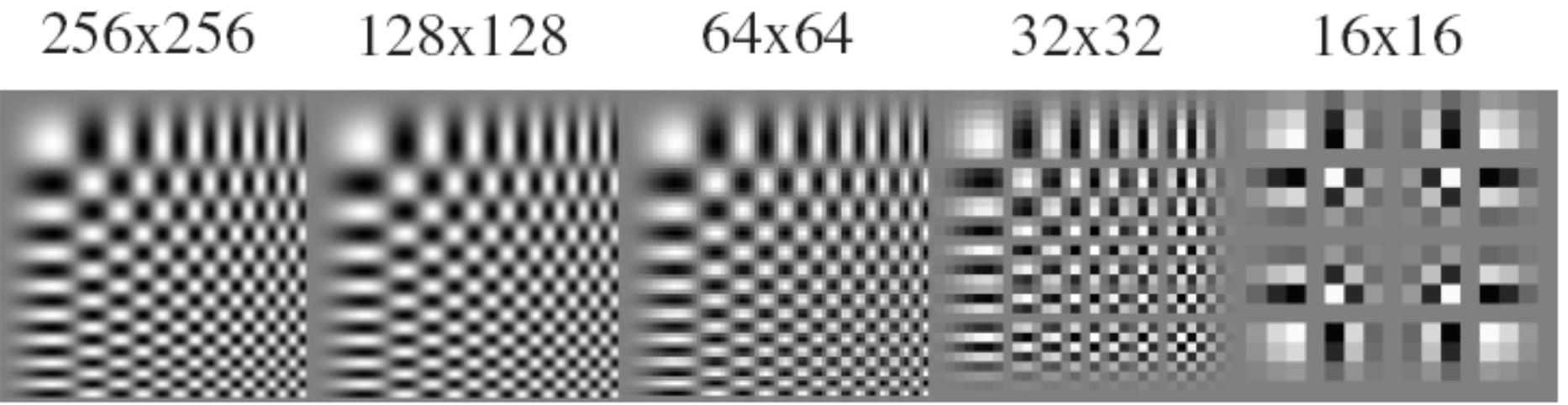
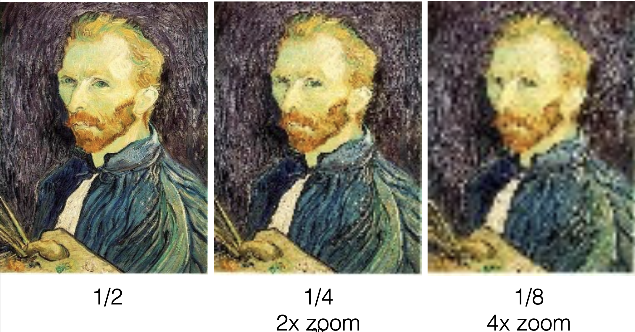
Aliasing

• Sub-sampling can result in aliasing artifacts
  • Wagon wheels rolling the wrong way in movies
  • Checkerboards disintegrate in ray tracing
  • Striped shirts look funn

Taken from CV lecture notes by (lost to history).

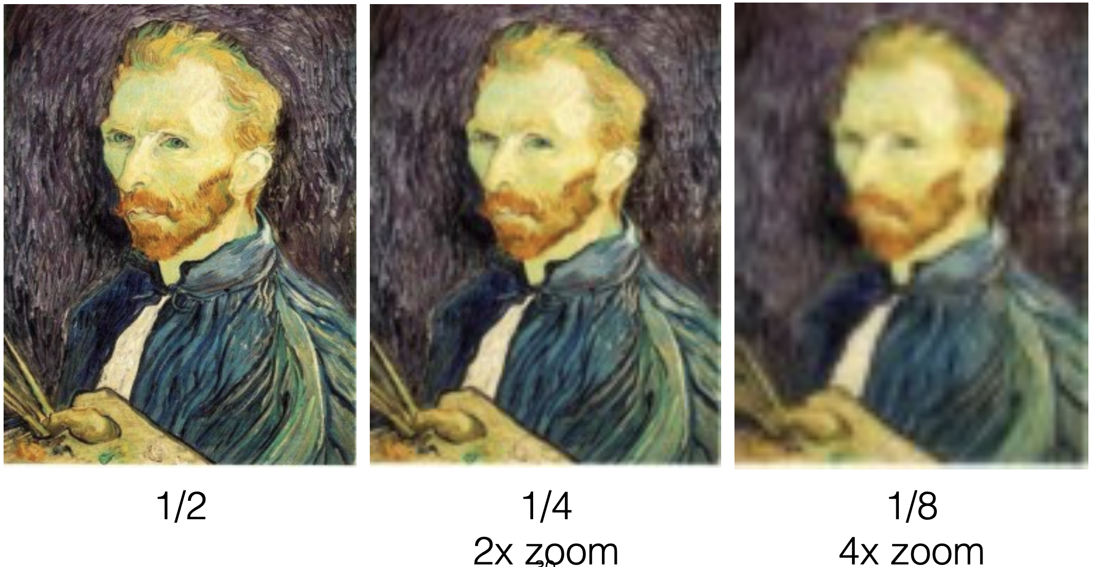
Anti-aliasing

• Sample more often
• Get rid of all frequency that are greater than half the sampling frequency
  • We will loose information
  • But still better than aliasing artifacts

Aliasing

Taken from CV lecture notes by (lost to history).

Anti-Aliasing

Taken from CV lecture notes by (lost to history).

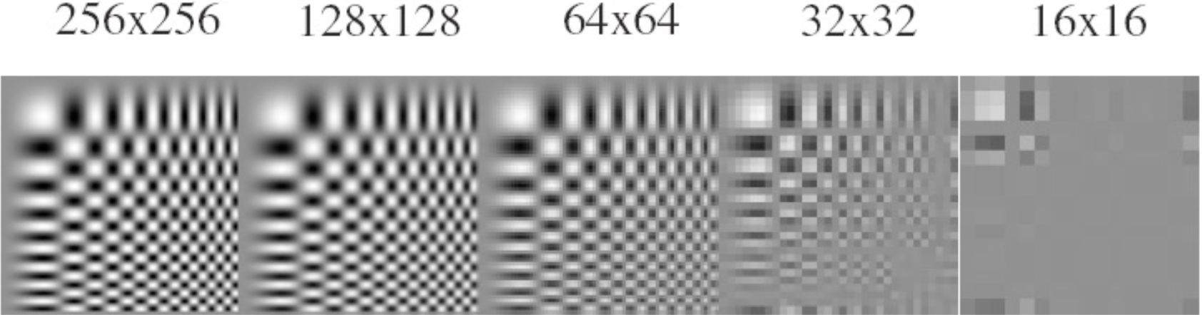
Without pre-filtering (i.e., without anti-aliasing)

Taken from CV lecture notes by (lost to history).

With pre-filtering

Taken from CV lecture notes by (lost to history).

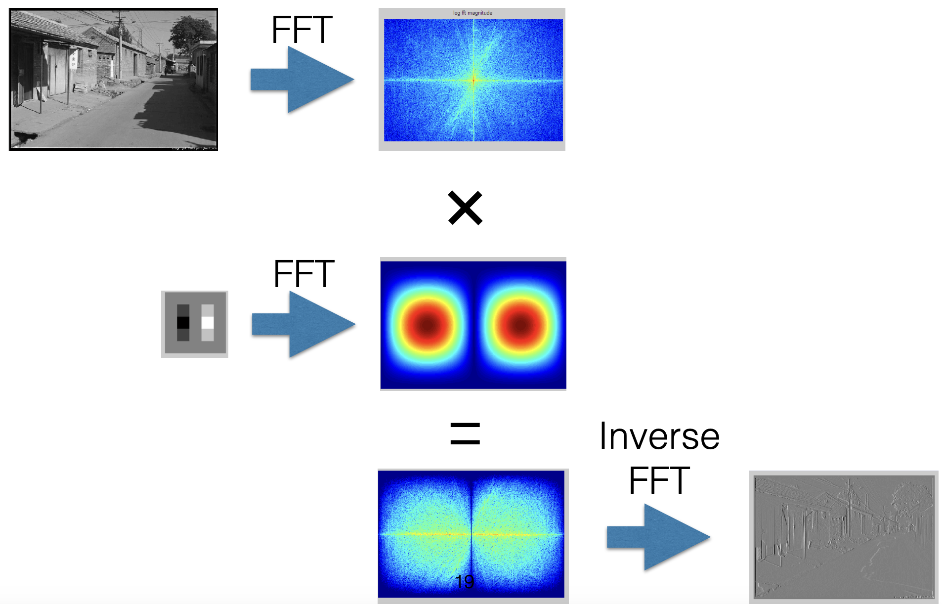
Convolution Theorem

Fourier transform of the convolution of two functions is the product of their Fourier transforms.

$$ \mathcal{F}\{g \ast h\} = \mathcal{F}\{g\} \mathcal{F}\{h\} $$

The inverse Fourier transform of the product of two Fourier transform is the convolution of the two inverse Fourier transforms.

$$ \mathcal{F}^{-1}\{g h\} = \mathcal{F}^{-1}\{g\} \ast \mathcal{F}^{-1}\{h\} $$

Convolution in spatial domain is equivalent to multiplication in frequency domain.

$$ \begin{array} \mathcal{F}^{-1} \{ \mathcal{F}\{g\} \mathcal{F}\{h\} \} &= \mathcal{F}^{-1}\{ \mathcal{F}\{g\} \} \ast \mathcal{F}^{-1}\{ \mathcal{F}\{h\} \} \\ &= g \ast h \end{array} $$

Taken from CV lecture notes by (lost to history).

Fourier Transform of an Image

import cv2 as cv

img = cv.imread('data/messi.jpg', 0)

plt.figure(figsize=(8,8))
plt.imshow(img, 'gray')
plt.title('Messi')
plt.xticks([])
plt.yticks([]);

img_fourier = np.fft.fft2(img)
img_fourier_shifted = np.fft.fftshift(img_fourier)
img_spectrum_magnitude = 20 * np.log(np.abs(img_fourier_shifted))

plt.figure(figsize=(8,8))
plt.imshow(img_spectrum_magnitude, cmap = 'gray')
plt.title('Fourier transform magnitude')
plt.xticks([])
plt.yticks([]);

Image Convolution using Fourier Transform

Step 1: Construct a 2D Gaussian kernel

import scipy.stats as st

def gkern(kernlen=5, sig=3):
    """Returns a 2D Gaussian kernel."""

    x = np.linspace(-kernlen/(3*sig), kernlen/(3*sig), kernlen+1)
    kern1d = np.diff(st.norm.cdf(x))
    kern2d = np.outer(kern1d, kern1d)
    return kern2d/kern2d.sum()

g = gkern(kernlen=11, sig=1)
plt.imshow(g)

<matplotlib.image.AxesImage at 0x113157890>

Step 2: Make this kernel the same size as the image by padding zeros

h, w = g.shape
g_resized = np.zeros(img.shape)
g_resized[:h,:w] = g

plt.figure(figsize=(8,8))
plt.imshow(g_resized)

<matplotlib.image.AxesImage at 0x11335c910>

Step 3: Take its Fourier Transform

g_fourier = np.fft.fft2(g_resized)
g_fourier_shifted = np.fft.fftshift(g_fourier)
g_spectrum_magnitude = 20 * np.log(np.abs(g_fourier_shifted))

plt.figure(figsize=(8,8))
plt.imshow(g_spectrum_magnitude, cmap = 'gray')
plt.title('Fourier transform magnitude')
plt.xticks([])
plt.yticks([]);

Step 4: Multiply the two fourier transforms

multiplied_fourier = img_fourier * g_fourier

Step 5: Take inverse Fourier transform.

img_filtered = np.real(np.fft.ifft2(multiplied_fourier))

plt.figure(figsize=(8,8))
plt.title('Convolution usinig Fourier Transform')
plt.imshow(img_filtered, cmap='gray');

Step 6: Lets confirm that we get the same result if we use convolution in spatial domain.

img_filtered2 =  sp.signal.convolve2d(img, g, mode='same', boundary='fill')

plt.figure(figsize=(8,8))
plt.title('Result using convolution in spatial domain')
plt.imshow(img_filtered2, cmap='gray');

Fourier Transform of Gaussiian vs. Averaging Kernel

g = gkern(kernlen=11, sig=1)
h, w = g.shape
g_resized = np.zeros(img.shape)
g_resized[:h,:w] = g
g_fourier = np.fft.fft2(g_resized)
g_fourier_shifted = np.fft.fftshift(g_fourier)
g_spectrum_magnitude = 20 * np.log(np.abs(g_fourier_shifted))

a = np.ones([11,11])/(11*11)
h, w = a.shape
a_resized = np.zeros(img.shape)
a_resized[:h,:w] = a
a_fourier = np.fft.fft2(a_resized)
a_fourier_shifted = np.fft.fftshift(a_fourier)
a_spectrum_magnitude = 20 * np.log(np.abs(a_fourier_shifted))

plt.figure(figsize=(15,9))
plt.subplot(221)
plt.xticks([])
plt.yticks([])
plt.title('Gaussian filter')
plt.imshow(g_resized)
plt.subplot(222)
plt.title('Averaging filter')
plt.imshow(a_resized)
plt.xticks([])
plt.yticks([])
plt.subplot(223)
plt.xticks([])
plt.yticks([])
plt.title('Fourier Transform of Gaussian filter')
plt.imshow(g_spectrum_magnitude, cmap='gray')
plt.subplot(224)
plt.xticks([])
plt.yticks([])
plt.title('Fourier Transform of averaging filter')
plt.imshow(a_spectrum_magnitude, cmap='gray')

<matplotlib.image.AxesImage at 0x1241dbc50>

img_with_gaussian =  sp.signal.convolve2d(img, g, mode='same', boundary='fill')
img_with_averaging =  sp.signal.convolve2d(img, a, mode='same', boundary='fill')

plt.figure(figsize=(15,9))
plt.subplot(221)
plt.xticks([])
plt.yticks([])
plt.title('Gaussian filter')
plt.imshow(img_with_gaussian, cmap='gray')
plt.subplot(222)
plt.title('Averaging filter')
plt.imshow(img_with_averaging, cmap='gray')
plt.xticks([])
plt.yticks([])
plt.subplot(223)
plt.xticks([])
plt.yticks([])
plt.title('Gaussian filter')
plt.imshow(img_with_gaussian[200:264,100:164], cmap='gray')
plt.subplot(224)
plt.title('Averaging filter')
plt.imshow(img_with_averaging[200:264,100:164], cmap='gray')
plt.xticks([])
plt.yticks([]);

Messing with frequencies

img = cv.imread('data/messi.jpg', 0)

img_fourier = np.fft.fft2(img)
img_fourier_shifted = np.fft.fftshift(img_fourier)
img_spectrum_magnitude = 20 * np.log(np.abs(img_fourier_shifted))

plt.figure(figsize=(8,8))
plt.imshow(img_spectrum_magnitude, cmap = 'gray')
plt.title('Fourier transform magnitude')
plt.xticks([])
plt.yticks([]);

rows, cols = img.shape
crow, ccol = rows//2, cols//2
how_much = 10

img_fourier_shifted2 = np.copy(img_fourier_shifted)
img_fourier_shifted2[crow-how_much:crow+how_much, ccol-how_much:ccol+how_much] = complex(1e-32)
img_spectrum_magnitude = 20 * np.log(np.abs(img_fourier_shifted2))

plt.figure(figsize=(8,8))
plt.imshow(img_spectrum_magnitude, cmap = 'gray')
plt.title('Fourier transform magnitude')
plt.xticks([])
plt.yticks([]);

img_fourier_unshifted = np.fft.ifftshift(img_fourier_shifted2)
img_back = np.fft.ifft2(img_fourier_unshifted)
img_back = np.abs(img_back)

plt.figure(figsize=(8,8))
plt.title('Result using convolution in spatial domain')
plt.imshow(img_back, cmap='gray');
plt.xticks([])
plt.yticks([])

([], [])

Why FFT?

When dealing with convolutions, it is often much faster to carry out these in the Fourier domain.

g = gkern(kernlen=64, sig=11)
plt.imshow(g)

<matplotlib.image.AxesImage at 0x124289a90>

# Image taken from https://cdn.hasselblad.com/samples/B0000835.jpg

i = cv.imread('data/big.jpg', 0)
plt.figure(figsize=(10,5))
plt.title('Image')
plt.imshow(i, cmap='gray');

%%time
g_resized = np.zeros(i.shape)
h, w = g.shape
g_resized[:h,:w] = g
g_fourier = np.fft.fft2(g_resized)

CPU times: user 1.32 s, sys: 273 ms, total: 1.59 s
Wall time: 1.59 s

Output:

CPU times: user 3.72 s, sys: 519 ms, total: 4.24 s
Wall time: 4.25 s

%%time
i_fourier = np.fft.fft2(i)
r = i_fourier*g_fourier
i_r = np.abs(np.fft.ifft2(r))

CPU times: user 2.77 s, sys: 368 ms, total: 3.13 s
Wall time: 3.14 s

Output:

CPU times: user 8.91 s, sys: 1.33 s, total: 10.2 s
Wall time: 10.3 s

plt.figure(figsize=(10,5))
plt.title('Gaussian blur via FFT')
plt.imshow(i_r, cmap='gray');

%%time
#
# This is very slow.  Run at your own peril.  Check out the times below.
i_r2 = sp.signal.convolve2d(i, g, mode='same', boundary='fill')

CPU times: user 4min 36s, sys: 631 ms, total: 4min 36s
Wall time: 4min 36s

Output:

CPU times: user 6min 36s, sys: 2.49 s, total: 6min 38s
Wall time: 6min 40s

# cv.imwrite('images/large-image-convolution.jpg', i_r2)

# We load the saved result

i_r3 = cv.imread('images/large-image-convolution.jpg')
plt.figure(figsize=(10,5))
plt.title('Gaussian blur without FFT')
plt.imshow(i_r3, cmap='gray');

plt.figure(figsize=(15,7))
plt.subplot(1,2,1)
plt.title('Gaussian blur with FFT')
plt.imshow(i_r, cmap='gray')
plt.xticks([])
plt.yticks([])
plt.subplot(1,2,2)
plt.title('Gaussian blur without FFT')
plt.xticks([])
plt.yticks([])
plt.imshow(i_r3, cmap='gray');

Hybrid images

Taken from CV lecture notes by (lost to history).

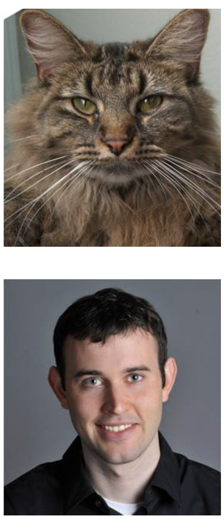
From afar

Taken from CV lecture notes by (lost to history).

When you are close

Taken from CV lecture notes by (lost to history).

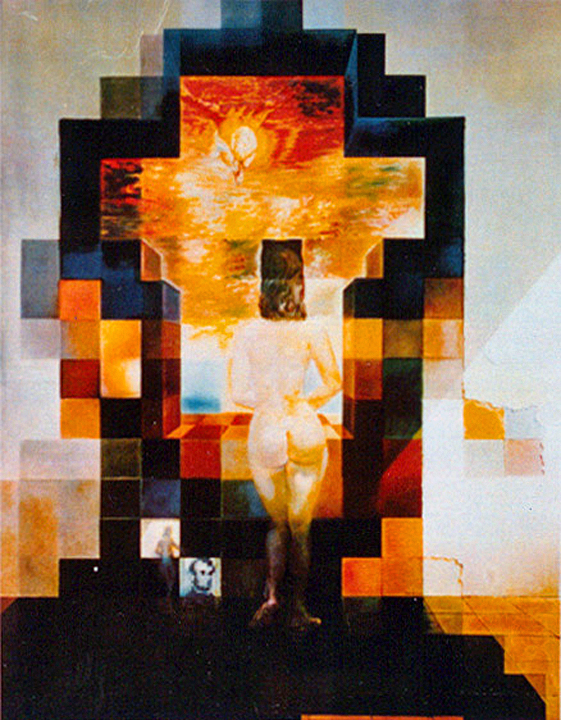
Example

• Dali Theater-Museum in Figueres, Spain.
• Gala Nude Abraham Lincoln by Salvador Dali.

From afar

Taken from CV lecture notes by (lost to history).

When you get closer

Taken from CV lecture notes by (lost to history).

Summary

• Fourier transform
• Image filtering in frequency domain
• Images are smooth (image compression?)
• Low-pass filternig before sampling
• Nyquist Theorem