
Image formation and pinhole camera model
Faisal Qureshi
Professor
Faculty of Science
Ontario Tech University
Oshawa ON Canada
http://vclab.science.ontariotechu.ca
Copyright information
© Faisal Qureshi
License

This work is licensed under a Creative Commons Attribution-NonCommercial 4.0 International License.
import numpy as np
import math
from scipy import linalg
Lesson Plan
- Pinhole camera model
- Homoegenous coordinates
- Intrinsic and extrinsic camera matrices
- Lens effects
- Camera calibration
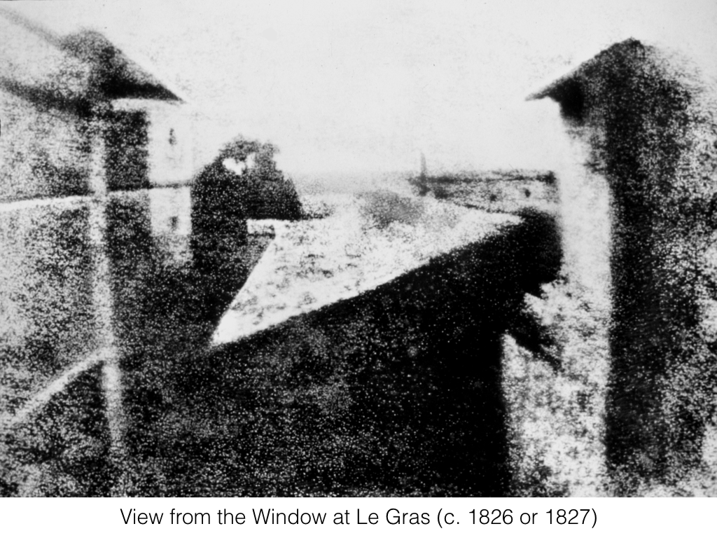
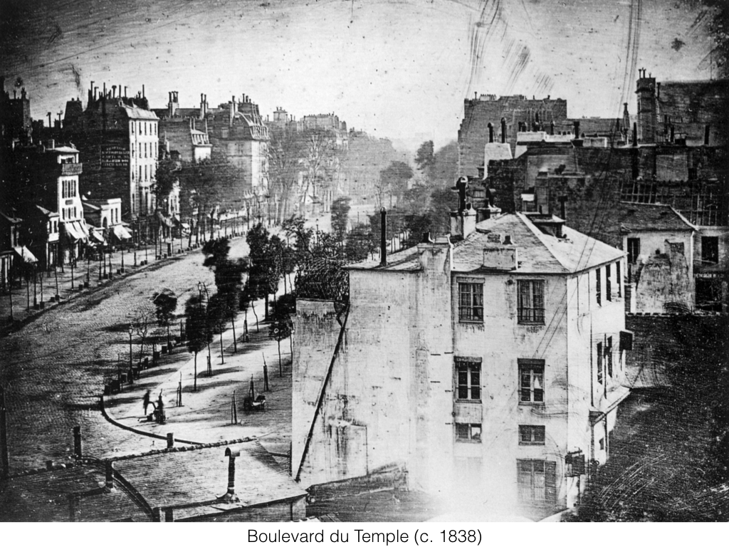
Examples of early photographs
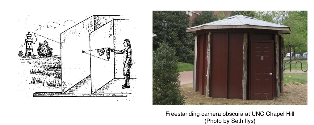
Camera Obscura
Known during the Classical Period (e.g., China c. 470BC)
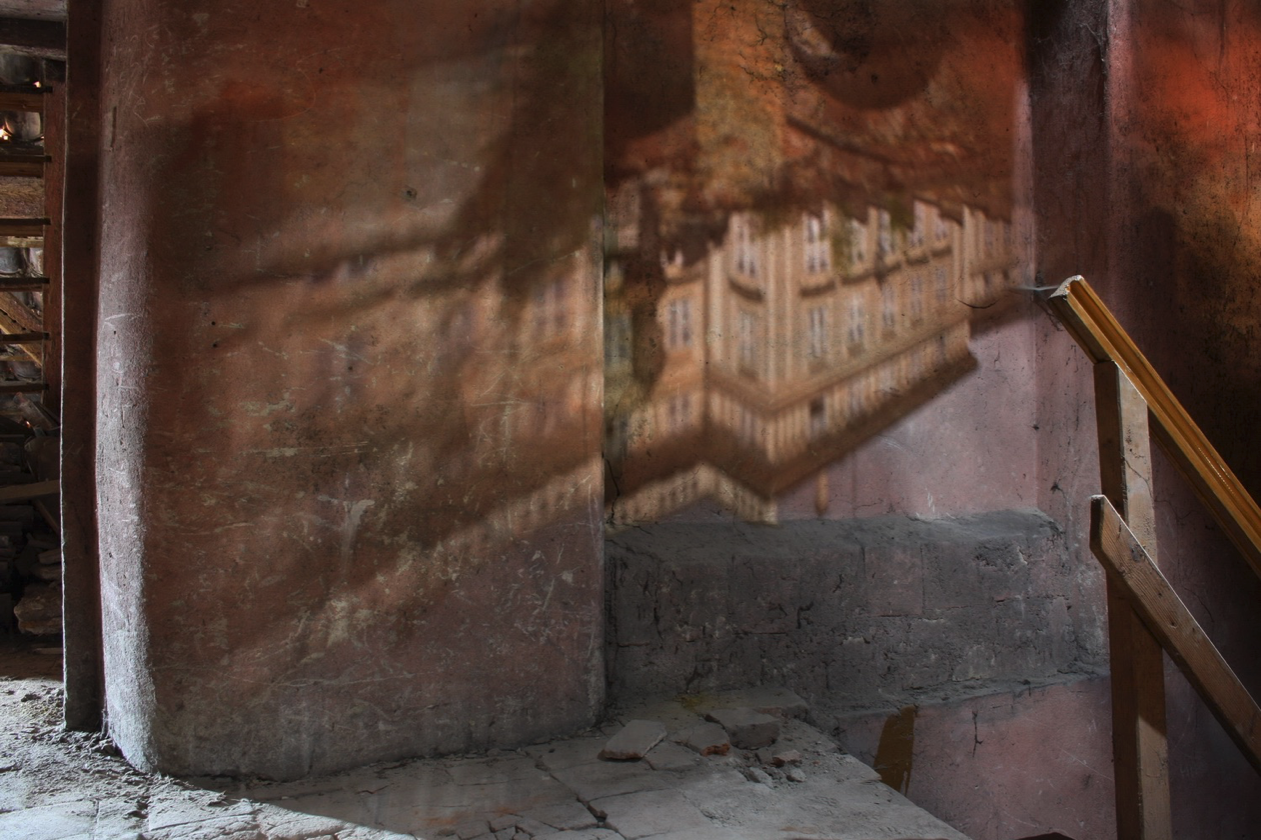
Outside scene imaged on a wall in Prague Castle. This probably occured due to a small crack on the opposite wall.
Pinhole Camera Model
In 2D
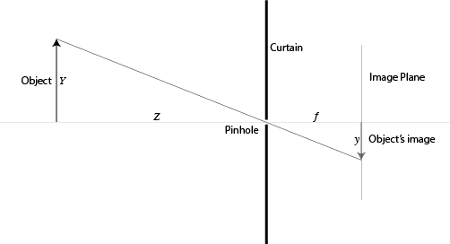
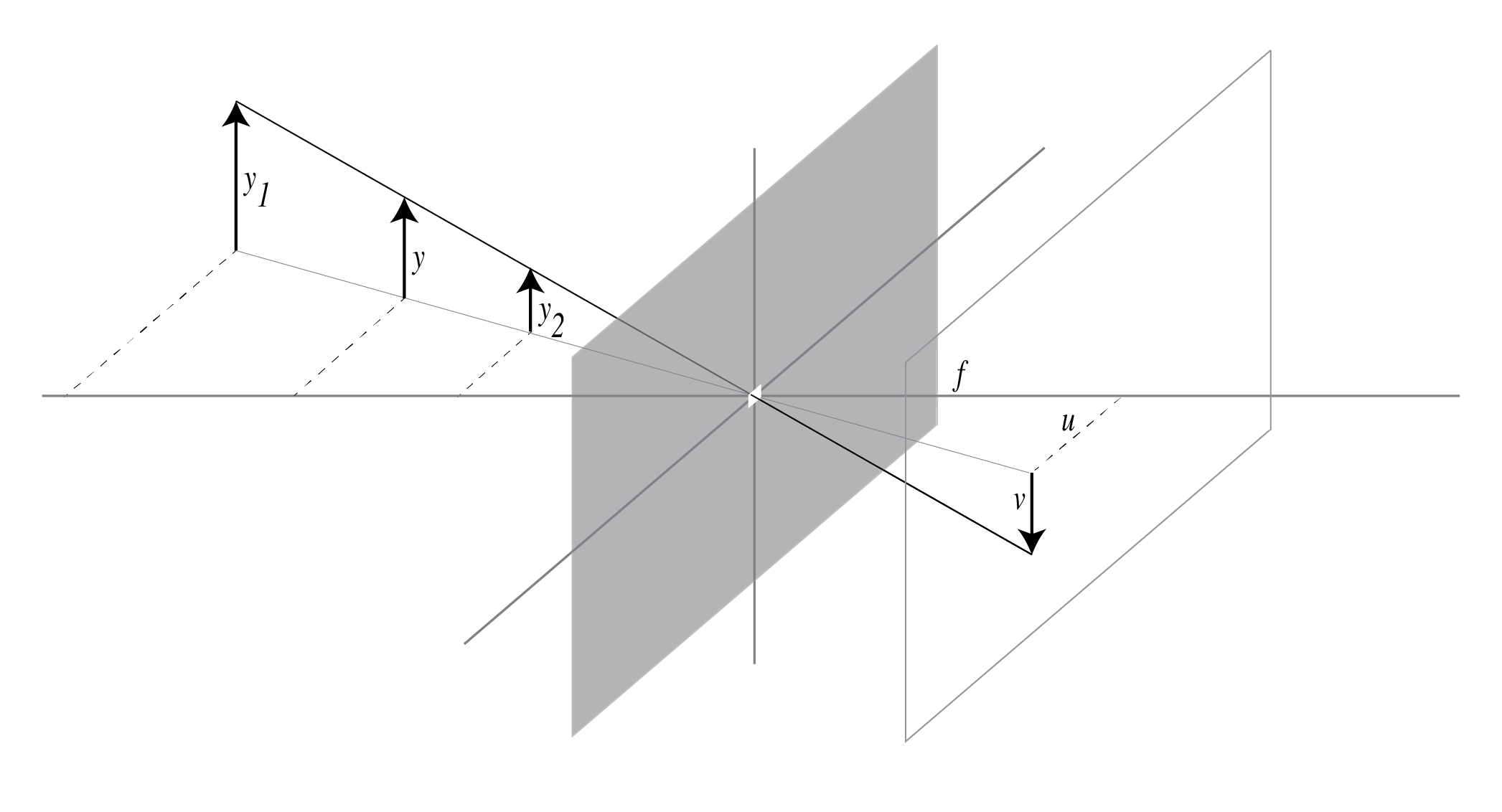
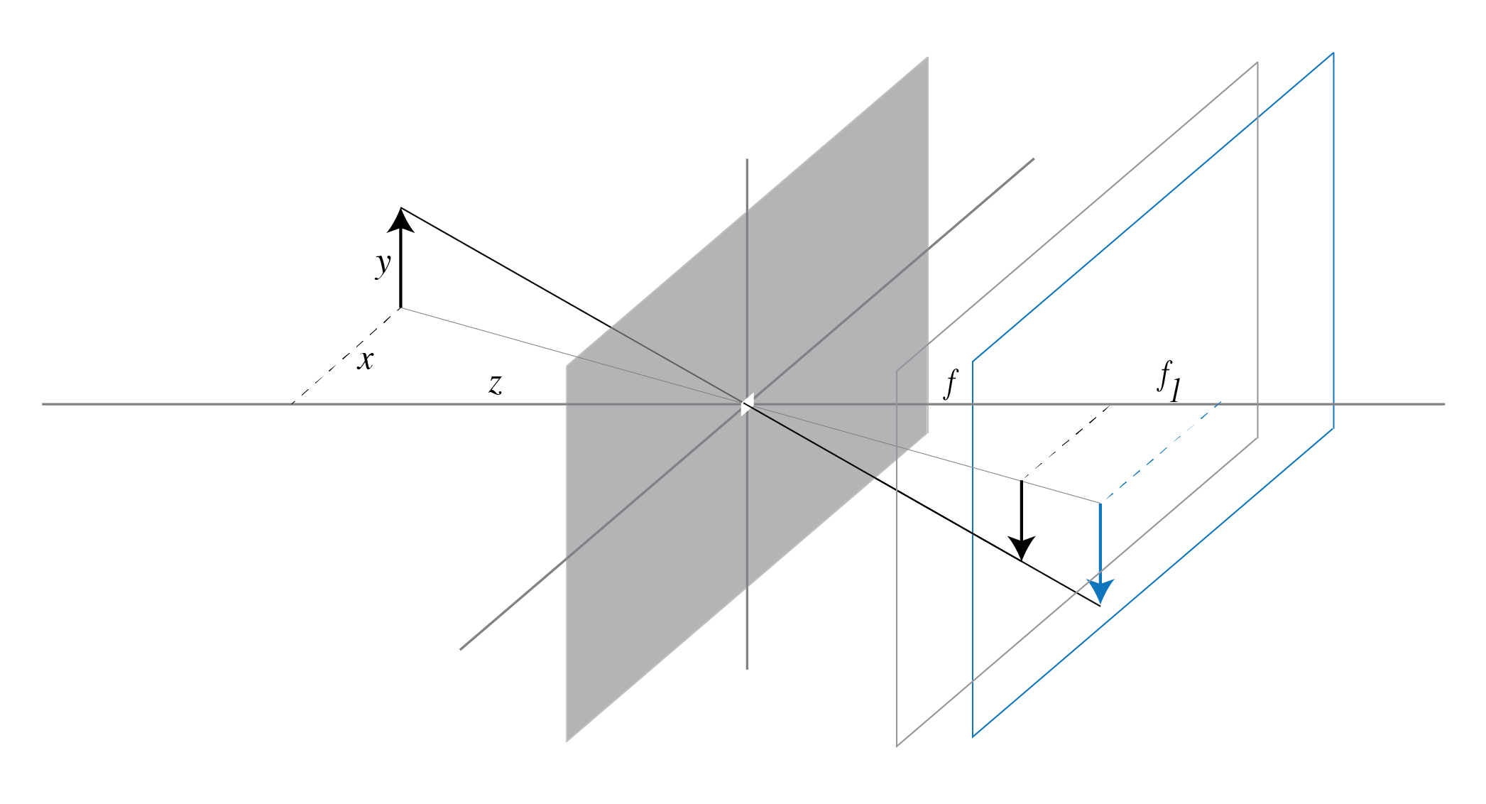
Given $Y$, the height of the object, $Z$, its distance from the pinhole, and $f$, the distance between the pinhole and the image plane (also known as the focal length), we want to estimate $y$, the height of the image of this object.
Using the similar triangles argument, we get
$$ Y / Z = y / f. $$
Re-arranging the above expression yields
$$ y = f Y / Z. $$
In 3D
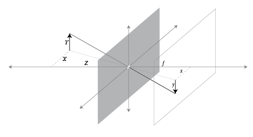
Pinhole model describes the relationship between a 3d point $(X,Y,Z)$ and its imaging location $(x,y)$. Here $f$ is the distance of the image plane and the pinhole, also known as the focal length, and $Z$ is the distance of the point from the pinhole. This formulation assumes that pinhole is situated at location $(0,0,0)$, or the origin, and the camera's optical axis is aligned with the global z-axis.
$$ \left( \begin{array}{c} X \\ Y \\ Z \end{array} \right) \longmapsto \left( \begin{array}{c} fX/Z \\ fY/Z \\ f \end{array} \right) \leadsto \left( \begin{array}{c} fX/Z \\ fY/Z \end{array} \right) $$
Homogeneous Coordinates
From Cartesian Coordinates to Homogeneous Coordinates
$$ \begin{array}{rcl} (x,y) & \to & (x,y,1) \\ (x,y,z) & \to & (x,y,z,1) \\ \end{array} $$
Example
$$ \begin{array}{rcl} (2,3) & \to & (2,3,1) \\ (10,-4,-2) & \to & (10,-4,-2,1) \\ \end{array} $$
From Homogeneous Coordinates to Cartesian Coordinates
$$ \begin{array}{rcl} (x,y,w) & \to & \left( x/w,y/w \right) \\ (x,y,z,w) & \to & \left( x/w,y/w,z/w \right) \\ \end{array} $$
Example
$$ \begin{array}{rcl} (6,-2,2) & \to & (3,-1) \\ (9,-24,-3,-3) & \to & (-3,8,1) \\ \end{array} $$
Homogeneous Coordinates Properties
Invariant to Scaling, i.e., $(x,y,w) = k(x,y,w)$. Both $(x,y,w)$ and $(kx, ky, kw)$ represent the same 2D Cartesian point $(x/w, y/w)$.
A Line in 2D Passing Through Two Points
Consider two 2D Cartesian points $(x_1,y_1)$ and $(x_2,y_2)$. We can find the line that passes through these points using cross-product in homogeneous coordinates.
Recall that equation of a line is $ax + by+c = 0$ then $$ (a,b,c) = (x_1,y_1,1) \times (x_2,y_2,1) $$
Proof
If line $a x + b y + c = 0$ satisfies points $(x_1, y_1)$ and $(x_2, y_2)$ then the following must be true
$$ \begin{align} a x_1 + b y_1 + c &= 0 \\ a x_2 + b y_2 + c &= 0 \\ \end{align} $$
We can re-write these equations in terms of the dot product of two vectors $\left[ \begin{array}{ccc} a & b & c \end{array} \right] \left[ \begin{array}{c} x_1 \\ y_1 \\ 1 \end{array} \right] = 0$ and $\left[ \begin{array}{ccc} a & b & c \end{array} \right] \left[ \begin{array}{c} x_2 \\ y_2 \\ 1 \end{array} \right] = 0$. The dot product of two vectors is only zero if the two vectors are perpendicular to each other. This suggests that vector $\left[ \begin{array}{ccc} a & b & c \end{array} \right]$ is perpendicular to both $\left[ \begin{array}{ccc} x_1 & y_1 & 1 \end{array} \right]$ and $\left[ \begin{array}{ccc} x_2 & y_2 & 1 \end{array} \right]$.
Given two vectors, their cross-product returns a vector that is perpendicular to both vectors. Consequently, we can compute $\left[ \begin{array}{ccc} a & b & c \end{array} \right]$ by taking a cross-product of vectors $\left[ \begin{array}{ccc} x_1 & y_1 & 1 \end{array} \right]$ and $\left[ \begin{array}{ccc} x_2 & y_2 & 1 \end{array} \right]$.
Exercise: computing a representation of a line from homogenous coordinates
Find a representation of the line between points $\mathbf{a}=(1,2)$ and $\mathbf{b}=(4,3)$ using homogeneous coordinates.
Solution
ah = np.array([1,2,1])
bh = np.array([4,3,1])

l = np.cross(ah, bh)
print('l = {}'.format(l))
print('Computed line passes through point a: {}'.format(math.isclose(np.dot(ah, l), 0.0)))
print('Computed line passes through point b: {}'.format(math.isclose(np.dot(bh, l), 0.0)))
l = [-1  3 -5]
Computed line passes through point a: True
Computed line passes through point b: True
Intersecting Lines
Given two lines $a_1 x + b_1 y + c_1=0$ and $a_2 x + b_2 y + c_2=0$, we can compute their intersection using cross-product as follows:
Step 1: Find intersection point in homogeneous coordinates
$$ (x,y,w) = (a_1,b_1,c_1) \times (a_2,b_2,c_2) $$
Step 2: Compute Cartesian coordinates from homogeneous coordinates
Intersection point is then $(x/w,y/w)$
Proof
Along the similar lines as before.
Example: finding the intersection of two lines using homogeneous coordinates
Use homogeneous coordinates to determine the intersection location for the following two lines.
$$ \begin{align} 3x - y + 7 & = 0 \\ 2x - y + 1 & = 0 \end{align} $$
l1 = np.array([3,-1,7])
l2 = np.array([2,-1,1])

ph = np.cross(l1, l2)
print('ph = {}'.format(ph))

p = ph[:2] / ph[2]
print('p = {}'.format(p))
print('Point p sits on l1: {}'.format(math.isclose(np.dot(l1, np.append(p,[1])), 0.0)))
print('Point p sits on l2: {}'.format(math.isclose(np.dot(l2, np.append(p,[1])), 0.0)))
ph = [ 6 11 -1]
p = [ -6. -11.]
Point p sits on l1: True
Point p sits on l2: True
Exercise: finding the intersection of two lines using homogeneous coordinates
Find intersection location for the following two lines.
$$ \begin{align} 3x - y + 7 & = 0 \\ 3x - y - 3 & = 0 \end{align} $$
Solution:
ah = np.array([3,-1,7])
bh = np.array([3,-1,-3])

p = np.cross(ah, bh)
print('p = {}'.format(p))
print('Homogenous component of p: w = {}'.format(p[2]))
print('Computed line passes through point a: {}'.format(math.isclose(np.dot(ah, p), 0.0)))
print('Computed line passes through point b: {}'.format(math.isclose(np.dot(bh, p), 0.0)))
p = [10 30  0]
Homogenous component of p: w = 0
Computed line passes through point a: True
Computed line passes through point b: True
Parallel Lines
$w=0$ if two lines are parallel. We say that these lines intersect at infinity. This suggests that it is possible to represent points at infinity in homogeneous coordinates. Just set the homogeneous coordinate to $0$.
Points at Infinity
We can represent a point at infinity by setting its $w=0$. E.g., Homogeneous coordinate $(3,-1,3,0)$ represents a point at infinity in the direction $(3,-1,3,0)$.
2D Transformations
Translation
\begin{aligned} \begin{pmatrix} x' \\ y' \end{pmatrix} = \begin{pmatrix} x \\ y \end{pmatrix} + \begin{pmatrix} t_x \\ t_y \end{pmatrix} \end{aligned}
and using homoegeneous coordinates allows us to represent translation as a matrix product
\begin{aligned} \begin{bmatrix} x' \\ y' \\ 1 \end{bmatrix} &= \begin{bmatrix} 1 & 0 & t_x \\ 0 & 1 & t_y \\ 0 & 0 & 1 \\ \end{bmatrix} \begin{bmatrix} x \\ y \\ 1 \end{bmatrix} = \mathbf{T} \begin{bmatrix} x \\ y \\ 1 \end{bmatrix} \end{aligned}
Scaling
\begin{aligned} \begin{bmatrix} x' \\ y' \end{bmatrix} = \begin{bmatrix} s_x & 0 \\ 0 & s_y \end{bmatrix} \begin{bmatrix} x \\ y \end{bmatrix} \end{aligned}
Using homoegeneous coordinates we get
\begin{aligned} \begin{bmatrix} x' \\ y' \\ 1 \end{bmatrix} = \begin{bmatrix} s_x & 0 & 0 \\ 0 & s_y & 0 \\ 0 & 0 & 1 \\ \end{bmatrix} \begin{bmatrix} x \\ y \\ 1 \end{bmatrix} &= \mathbf{S} \begin{bmatrix} x \\ y \\ 1 \end{bmatrix} \end{aligned}
Rotation
\begin{aligned} \begin{bmatrix} x' \\ y' \end{bmatrix} = \begin{bmatrix} \cos(\theta) & -\sin(\theta) \\ \sin(\theta) & \cos(\theta) \end{bmatrix} \begin{bmatrix} x \\ y \end{bmatrix} \end{aligned}
Using homogeneous coordinates we get
\begin{aligned} \begin{bmatrix} x' \\ y' \\ 1 \end{bmatrix} = \begin{bmatrix} \cos(\theta) & -\sin(\theta) & 0 \\ \sin(\theta) & \cos(\theta) & 0 \\ 0 & 0 & 1 \\ \end{bmatrix} \begin{bmatrix} x \\ y \\ 1 \end{bmatrix} = \mathbf{R} \begin{bmatrix} x \\ y \\ 1 \end{bmatrix} \end{aligned}
Shearing
\begin{aligned} \begin{bmatrix} x' \\ y' \end{bmatrix} = \begin{bmatrix} 1 & q_x \\ q_y & 1 \end{bmatrix} \begin{bmatrix} x \\ y \end{bmatrix} \end{aligned}
Using homogeneous coordinates we get
\begin{aligned} \begin{bmatrix} x' \\ y' \\ 1 \end{bmatrix} = \begin{bmatrix} 1 & q_x & 0 \\ q_y & 1 & 0 \\ 0 & 0 & 1 \\ \end{bmatrix} \begin{bmatrix} x \\ y \\ 1 \end{bmatrix} = \mathbf{Q} \begin{bmatrix} x \\ y \\ 1 \end{bmatrix} \end{aligned}
Chaining transformations
By representing each transformation as a matrix-vector product, we can easily chain multiple transformations together. Note also that without using homogeneous coordinates, we cannot represent translation as a matrix-vector product. It is for this reason that homogeneous coordinates are extensively used in computer graphics and vision when dealing with scene and camera geometry.
Example
import matplotlib.pyplot as plt
import numpy as np

points_original = np.array([
    [0, 0, 1],
    [1, 0, 1],
    [1, 1, 1],
    [0, 1, 1],
    [0, 0, 1]  # Repeat the first point to close the shape for plotting
]).T # Transpose so columns are points

tx, ty = 1, 3
T = np.array([
    [1, 0, tx],
    [0, 1, ty],
    [0, 0, 1]
])

sx, sy = 0.5, 2.5
S = np.array([
    [sx, 0, 0],
    [0, sy, 0],
    [0, 0, 1]
])

theta = 25.0 * np.pi / 180.0
R = np.array([
    [np.cos(theta), -np.sin(theta), 0],
    [np.sin(theta), np.cos(theta), 0],
    [0, 0, 1]
])

qx, qy = 1, 4
Q = np.array([
    [1, qx, 0],
    [qy, 1, 0],
    [0, 0, 1]
])

points_transformed_homo =  R @ points_original
points_transformed = points_transformed_homo / points_transformed_homo[2, :]

# 5. Plotting
plt.figure(figsize=(7, 7))

# Plot Original
plt.subplot(1, 1, 1)
plt.plot(points_original[0, :], points_original[1, :], '-o', color='blue', label='Original')
plt.fill(points_original[0, :], points_original[1, :], alpha=0.1, color='blue')
plt.plot(points_transformed[0, :], points_transformed[1, :], '-o', color='red', label='Transformed')
plt.fill(points_transformed[0, :], points_transformed[1, :], alpha=0.1, color='red')
plt.grid(True)
plt.legend()
plt.xlim([-10,10])
plt.ylim([-10,10])
plt.show()
Back to Pinhole Model
We now develop a mathematical model for pinhole cameras. This discussion follows Ch. 6 of Multiple View Geometry in Computer Vision (2nd Ed.) by Harley and Zisserman. For the following discussion we assume the following camera geometry.
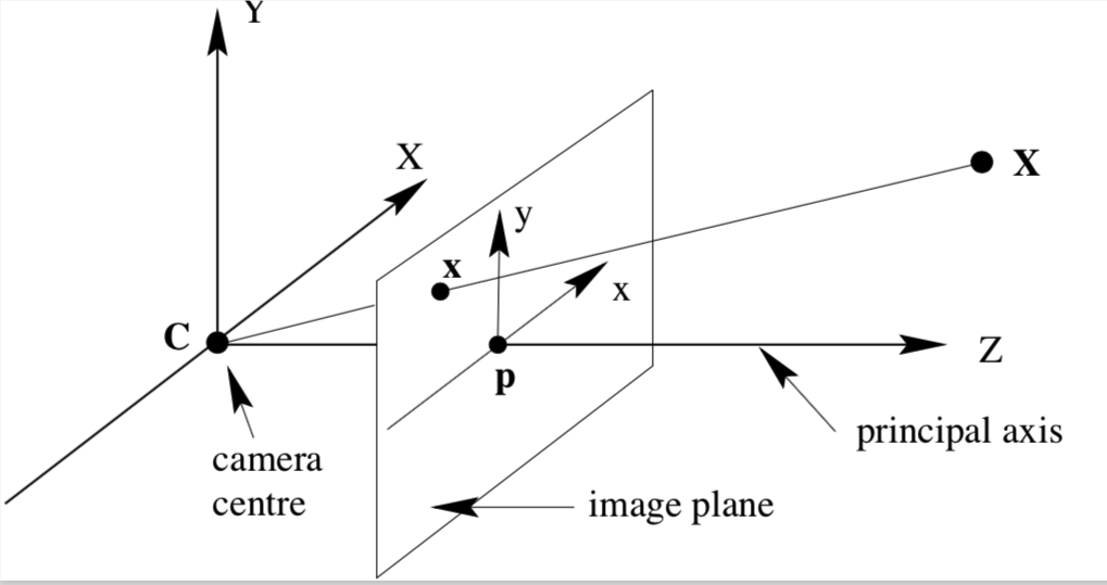
This assumes that the image plane sits in front of the pinhole. Obviously, no physical camera has this property. Never the less it is mathematically convenient (and equivalent) to model pinhole cameras as such.
- Camera centre sits at the origin of the Euclidean coordinate system Camera centre is also known as center of projection or optical centre
- Image plane (also known as the focal plane) sits at $Z = f$
- Point in 3D space $$ \mathbf{X} = (X, Y, Z)^T $$
- This point is mapped to $$ \left( f X / Z, f Y / Z, f \right) $$
- Image coordinates are (just drop $f$) $$ \left( f X / Z, f Y / Z \right) $$
- Principal axis or principal ray is the line perpendicular to the image plane and passing through the centre of projection
- Principal point is the intersection location of image plane with the principal axis
- Principal plane is parallel to the image plane and passes through the centre of projection
Using Homoegenous Coordinates
We can describe the pinhole camera model using homoegenous coordinates as follows
$$ \begin{align} \left( \begin{array}{c} X \\ Y \\ Z \\ 1 \end{array} \right) \longmapsto \left( \begin{array}{c} fX \\ fY \\ Z \end{array} \right) & = \left[ \begin{array}{cccc} f & & & 0 \\ & f & & 0 \\ & & 1 & 0 \end{array} \right] \left( \begin{array}{c} X \\ Y \\ Z \\ 1 \end{array} \right) \\ & = \mathrm{diag}(f,f,1)\left[\mathbf{I}\ |\ \mathbf{0}\right] \left( \begin{array}{c} X \\ Y \\ Z \\ 1 \end{array} \right) \end{align} $$
We set
$$ \mathtt{P} = \mathrm{diag}(f,f,1)\left[\mathbf{I}\ |\ \mathbf{0}\right] $$
to denote the projection matrix. Specifically, we use $\mathtt{P}$ to map 3D points $\mathbf{X}$ to image points $\mathbf{x}$:
$$ \mathbf{x} = \mathtt{P} \mathbf{X}. $$
Under these assumptions, $\mathtt{P}$ has one degree-of-freedom, namely, the parameter $f$.
Principal Point Offset
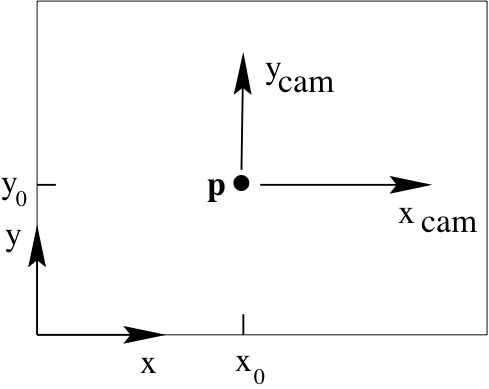
The above discussion assumes that the principle point sits at the origin of the coordinates in the image plane. Lets relax this assumption. Say $(p_x, p_y)$ are the coordinates of the principal point. Then
$$ \begin{align} \left( \begin{array}{c} X \\ Y \\ Z \\ 1 \end{array} \right) \longmapsto \left( \begin{array}{c} fX + p_x Z \\ fY + p_y Z \\ Z \end{array} \right) & = \left[ \begin{array}{cccc} f & & p_x & 0 \\ & f & p_y & 0 \\ & & 1 & 0 \end{array} \right] \left( \begin{array}{c} X \\ Y \\ Z \\ 1 \end{array} \right) \\ & = \mathbf{K} \left[\mathbf{I}\ |\ \mathbf{0}\right] \mathbf{X}_{\mathtt{cam}} \end{align} $$
Note $\mathbf{X}_{\mathtt{cam}}$. This captures our assumption that the camera centre is located at the origin of the Euclidean coordinate system (we can think of this as the world coordinate system) with camera pointing straight down the $z$-axis. $\mathbf{X}_{\mathtt{cam}}$ denotes that the point is expressed in the camera coordinate system.
In this case, we set projection matrix to
$$ \mathtt{P} = \mathbf{K} \left[\mathbf{I}\ |\ \mathbf{0}\right] $$
Exercise: Degrees of freedom of a projection matrix
How many degrees of freedom does a projection matrix have when the camera centre is assumed to be fixed at the origin with the camera pointing straight down the $z$-axis? That is, how many parameters are required to specify a projection matrix $\mathtt{P}$ uniquely under these assumptions?
Solution:
In this case, the matrix $\mathtt{P}$ has three degrees of freedom (captured in the parameters $f$, $p_{x}$, and $p_{y}$).
(From solutions/image-formation/solution_03.md)
Camera Rotation and Translation
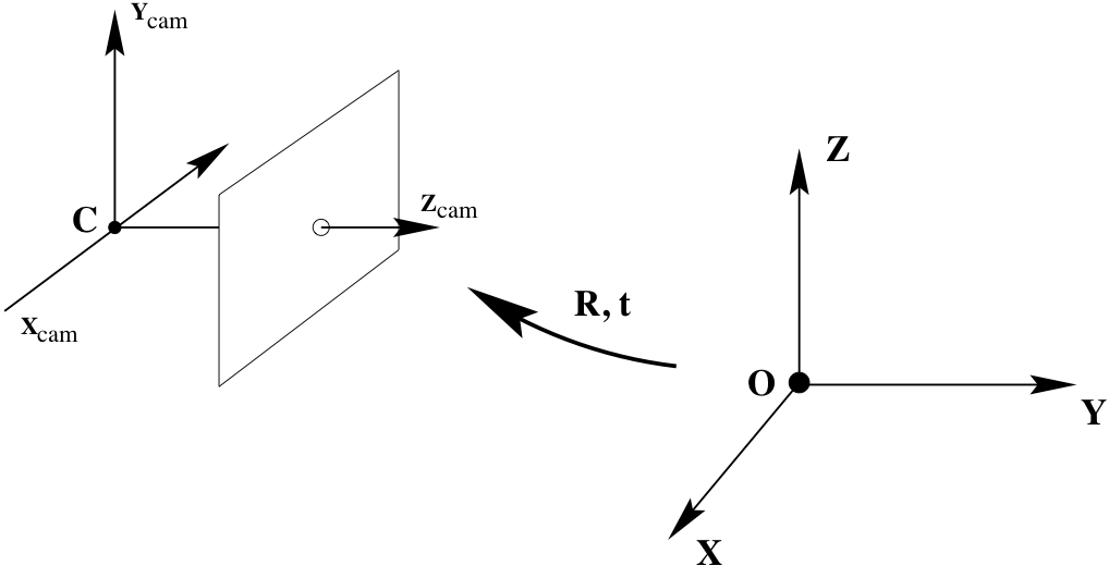
Now we relax our assumption that the camera centre is located at the origin of the Euclidean coordinate system (we can think of this as the world coordinate system) with camera pointing straight down the $z$-axis.
Say camera centre in Cartesian coordinates is $\tilde{\mathbf{C}}$ and that camera rotation is represented by matrix $\mathbf{R}$. Then we can transform a Cartesian point $\tilde{\mathbf{X}}$ in the world coordinate system to a Cartesian point $\tilde{\mathbf{X}}_{\mathtt{cam}}$ in the camera coordinates system as follows
$$ \tilde{\mathbf{X}}_{\mathtt{cam}} = \mathbf{R} \left( \tilde{\mathbf{X}} - \tilde{\mathbf{C}} \right) $$
We can re-write this as follows
$$ \mathbf{X}_{\mathtt{cam}} = \left[ \begin{array}{cc} \mathbf{R} & - \mathbf{R} \tilde{C} \\ \mathbf{0} & 1 \end{array} \right] \left( \begin{array}{c} X \\ Y \\ Z \\ 1 \end{array} \right) $$
Putting it all together
$$ \mathbf{x} = \mathbf{K} \mathbf{R} \left[\mathbf{I}\ |\ -\tilde{C}\right] \mathbf{X} $$
It is often convenient to set $\mathbf{t} = -\mathbf{R} \tilde{C}$. Then we can rewrite the above as follows
$$ \mathbf{x} = \mathbf{K} \left[\mathbf{R}\ |\ \mathbf{t} \right] \mathbf{X} $$
In this case, we set projection matrix to
$$ \mathtt{P} = \mathbf{K} \left[\mathbf{R}\ |\ \mathbf{t} \right] $$
A note about camera rotation matrix $\mathbf{R}$
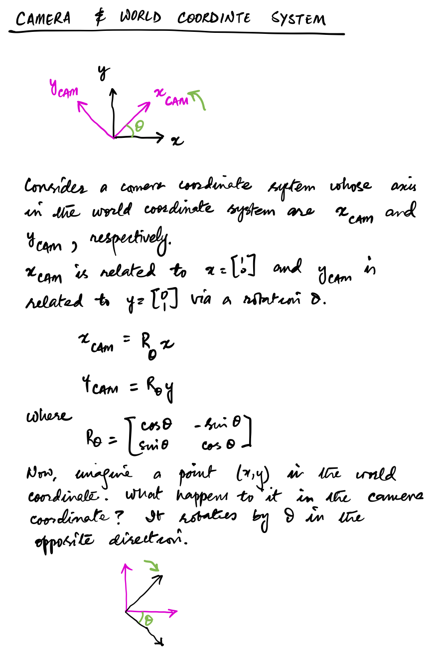
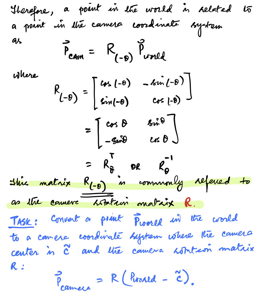
Exercise: Degrees of freedom of a projection matrix
How many degrees of freedom does a projection matrix have when the camera centre is assumed to be fixed at $\tilde{\mathbf{C}}$ and the camera's rotation is represented by matrix $\mathbf{R}$? That is, how many parameters are required to specify a projection matrix $\mathtt{P}$ uniquely under these assumptions?
Solution:
In this case, there are an additional three extrinsic parameters from the coordinates of $\mathbf{t} = -\mathbf{R} \tilde{C}$ and another three that determine the $3\times3$ rotation matrix $\mathbf{R}$. Thus, added to the three parameters $f$, $p_x$, and $p_y$ that determine the matrix $\mathbf{K}$, there are nine parameters required to determine the projection matrix $\mathtt{P}$.
(From solutions/image-formation/solution_04.mdsolutions/image-formation/solution_04.md)
CCD Pixel Sizes and Skew
Thus far we have assumed that image coordinates have equal scales in $x$ and $y$. If the number of pixels per unit distance in image coordinates are $m_x$ and $m_y$ in the $x$ and $y$ directions then we re-write $\mathbf{K}$ as follows
$$ \mathbf{K} = \left[ \begin{array}{ccc} \alpha_x & s & x_0 \\ & \alpha_y & y_0 \\ & & 1 \end{array} \right] $$
where $\alpha_x = f m_x$, $\alpha_y = f m_y$, $x_0 = m_x p_x$, $y_0 = m_y p_y$, $s$ is the skew term, which is often $0$. Note that $x_0$ and $y_0$ are the coordiantes of hte principal point in terms of pixel dimensions in $x$ and $y$ directions. $s$ becomes non-zero under special circumstances when lens is not aligned with the image plane.
Exercise: Degrees of freedom of a projection matrix
How many degrees of freedom does a projection matrix have when the camera centre is assumed to be fixed at $\tilde{\mathbf{C}}$ and the camera's rotation is represented by matrix $\mathbf{R}$ when the pixels are non-uniformly scaled as just described? That is, how many parameters are required to specify a projection matrix $\mathtt{P}$ uniquely under these assumptions?
Solution:
In this case, there are five parameters associated with the matrix $\mathbf{K}$, three with the coordinates of $\mathbf{t}$, and another three with the $3\times3$ rotation matrix $\mathbf{R}$. Thus, the projection matrix $\mathtt{P}$ has eleven degrees of freedom.
(From solutions/image-formation/solution_05.md)
Mapping 3D world points to 2D image poingts
We get the following equation that describes the mapping from world points to image points.
$$ \begin{align} \mathbf{x} & = \mathtt{P} \mathbf{X} \\ & = \mathbf{K} \left[ \mathbf{R}\ |\ \mathbf{t} \right] \mathbf{X} \end{align} $$
Note that $\mathtt{P}$ is the same as a homogeneous $3 \times 4$ matrix defined upto an arbitrary scale of rank 3. Projective matrices of rank less than 3 do not span the image plane. The projections might degenerate to a line or a point.
Extrinsic and Intrinsic matrices
We'll refer to $\mathtt{P}$ as the camera matrix.
Furthermore we refer to $\mathbf{K}$ as the intrinsic matrix, and $\left[ \mathbf{R}\ |\ \mathbf{t} \right]$ is the extrinsic matrix.
Note that
$$ \begin{align} \mathtt{P} = \mathbf{K} \left[ \mathbf{R}\ |\ \mathbf{t} \right] \end{align} $$
Properties of camera matrix $\mathtt{P}$
Recall from above that $\mathtt{P}$ projects 3D world points to 2D image points. Also that we work in homogeneous coordinates.
To make the following discussion easier, lets express $\mathtt{P}$ as
$$ \mathtt{P} = \left[ \mathtt{M}\ |\ \mathbf{p}_4 \right] $$
Here $\mathtt{M}$ is the top-left $3 \times 3$ submatrix of $\mathtt{P}$ and $\mathbf{p}_4$ is the last column of $\mathtt{P}$. Furthermore, let $\mathbf{p}^{iT}$ and $\mathbf{p}_j$ represent the $i$-th row and $j$-th column of $\mathtt{P}$, respectively. We can similarly denote rows and columns of $\mathtt{M}$.
Matrix $\mathtt{M}$
Recall that $ \mathtt{P} = \left[ \begin{array}{cccc} p_{11} & p_{12} & p_{13} & p_{14} \\ p_{21} & p_{22} & p_{23} & p_{24} \\ p_{31} & p_{32} & p_{33} & p_{34} \end{array} \right]. $ Let $ \mathtt{M} = \left[ \begin{array}{ccc} p_{11} & p_{12} & p_{13} \\ p_{21} & p_{22} & p_{23} \\ p_{31} & p_{32} & p_{33} \end{array} \right] $ and $ \mathbf{p}_4 = \left[ \begin{array}{c} p_{14} \\ p_{24} \\ p_{34} \end{array} \right]. $ Then $\mathtt{P} = \left[ \mathtt{M}\ |\ \mathbf{p}_4 \right].$
Finite Projective Camera
If $\mathtt{M}$ is non-singular then we have a finite projective camera. There are cases when $\mathtt{M}$ is singular. These are referred to as general projective cameras.
Thought experiment: what value of $x$ will satisfy the following equation.
$$ 2 * x - 8 = 0 $$
Camera Center
In general camera center is the right nullspace of matrix $\mathtt{P}$ since $\mathtt{P} \mathbf{C} = \mathbf{0}$.
Alternately, we can use the following to find the camera center
$$ \tilde{\mathbf{C}} = - \mathtt{M}^{-1} \left( \begin{array}{c} p_{14} \\ p_{24} \\ p_{34} \end{array} \right) $$
Recall that
$$ \mathbf{C} = \left( \tilde{C}^T, 1 \right)^T $$
Aside 1:
If $\mathtt{M}$ is singular (in case of general projective cameras), camera center (at infinity) is the right null space of $\mathtt{M}$, i.e., $\mathtt{M} \mathbf{d} = \mathbf{0}$. In this case,
$$ \mathbf{C} = \left( \mathbf{d}^T, 0 \right)^T $$
Aside 2:
The singular value decomposition (SVD) of a matrix $\mathtt{P}$ may be written as
$$ \mathtt{P} = \mathtt{U} \mathtt{\Sigma} \mathtt{V}^T $$
Then the (right) null space of $\mathtt{P}$ is the columns of $\mathtt{V}$ corresponding to singular values equal to zero.
Columns and rows of $\mathtt{P}$
Matrix $$ \mathtt{P} = \left[ \begin{array}{cccc} p_{11} & p_{12} & p_{13} & p_{14} \\ p_{21} & p_{22} & p_{23} & p_{24} \\ p_{31} & p_{32} & p_{33} & p_{34} \end{array} \right] $$ consits of 4 columns $$ \mathbf{p}_1 = \left[ \begin{array}{c} p_{11} \\ p_{21} \\ p_{31} \end{array} \right],\ \mathbf{p}_2 = \left[ \begin{array}{c} p_{12} \\ p_{22} \\ p_{32} \end{array} \right],\ \mathbf{p}_3 = \left[ \begin{array}{c} p_{13} \\ p_{23} \\ p_{33} \end{array} \right],\mathrm{\ and\ } \mathbf{p}_4 = \left[ \begin{array}{c} p_{14} \\ p_{24} \\ p_{34} \end{array} \right] $$
and 3 rows
$$ \begin{align} \mathbf{p}^{1T} & = \left[ \begin{array}{cccc} p_{11} & p_{12} & p_{13} & p_{14} \end{array} \right], \\ \mathbf{p}^{2T} &= \left[ \begin{array}{cccc} p_{21} & p_{22} & p_{23} & p_{24} \end{array} \right],\mathrm{\ and} \\ \mathbf{p}^{3T} &= \left[ \begin{array}{cccc} p_{31} & p_{32} & p_{33} & p_{34} \end{array} \right] \end{align} $$
Columns of $\mathtt{P}$
$\mathbf{p}_1$, $\mathbf{p}_2$ and $\mathbf{p}_3$ represent vanishing points in the $x$, $y$, and $z$ directions.
$\mathbf{p}_4$ is the image of the world origin.
Aside:
Homogeneous point $\mathbf{D} = (1,0,0,0)^T$ represent the $x$-axis. Then $\mathtt{P} \mathtt{D} = \mathbf{p_1}$ is the vanishing point in $x$-direction.
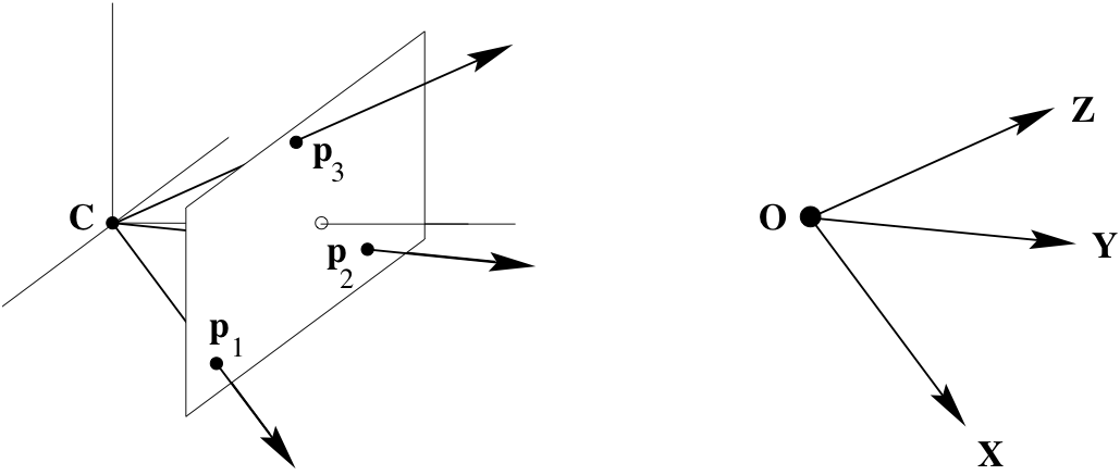
Rows of $\mathtt{P}$
$\mathbf{p}^{1T}$ and $\mathbf{p}^{2T}$ represent planes defined by the camera centre and image plane coordinate axis $x$ and $y$.
$\mathbf{p}^{3T}$ represents the principal plane.
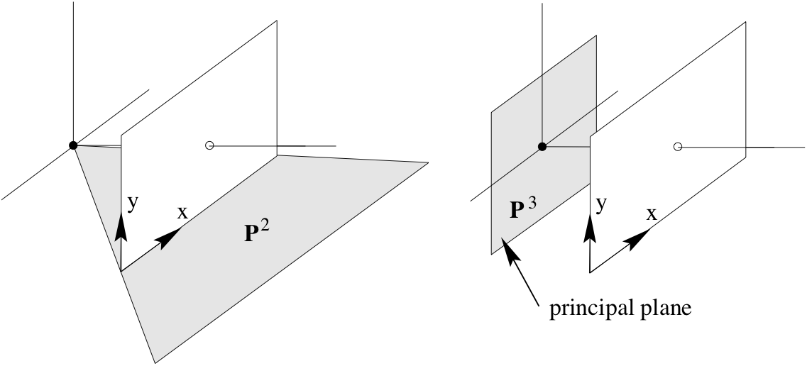
One way to convince ourselves that $\mathbf{p}^{3T}$ represents the principal plane is to see that the only way a point $\mathbf{X}$ maps to $(x,y,0)$ is if $\mathbf{p}^{3} \mathbf{X} = 0$. Similar arguments can be made for $\mathbf{p}^{1T}$ and $\mathbf{p}^{2T}$ representing planes defined by camera center and image plane cooridnate axis $x$ and $y$, respectively.
Principal Point
The principal point is given by $\mathtt{M} \mathbf{m}^{3}$, where $\mathbf{m}^{3T}$ is the third row of $\mathtt{M}$.
Aside:
Notice that the principal plane is given by $\mathbf{p}^{3T}$. The normal to this plane is $(p_{31}, p_{32}, p_{33})$ and using this information we can set a point at infinity using homogeneous coordinates as follows
$$ \hat{\mathbf{p}}^{3} = (p_{31}, p_{32}, p_{33}, 0) $$
Now project this point using $\mathtt{P}$ and we get the principal point.
Principal Axis Vector
$\mathbf{v} = \mathrm{det}(\mathtt{M}) \mathbf{m}^3$ is a vector in the direction of the principal axis, directed towards the front of the camera.
Action of $\mathtt{P}$ on points
Forward Projection
Points in the world are mapped to image coordinates using
$$ \mathbf{x} = \mathtt{P} \mathbf{X} $$
Points $\mathbf{D}=(\mathbf{d}^T,0)$ on the plane at infinity map to vanishing points in the image $\mathbf{x} = \mathtt{M} \mathbf{d}$
Back-projection of points to rays
Given a point $\mathbf{x}$ in the image, we seek to determine the set of points in space that map to this point. This set of points is a ray passing point $\mathtt{P}^+ \mathbf{x}$ and the camera centre.
$$ \mathbf{X}(\lambda) = \mathtt{P^+} \mathbf{x} + \lambda \mathbf{C} $$
Here $\mathtt{P}^+ = \mathtt{P}^T \left( \mathtt{P} \mathtt{P}^T \right)^{-1}$ is the psuedo-inverse of $\mathtt{P}$. Note that $\mathtt{P} \mathtt{P}^+ = \mathbf{I}$.
For finite cameras, we can develop a simpler expression. Recall that camera centre for these cameras is given by $\tilde{\mathbf{C}} = - \mathtt{M}^{-1} \mathbf{p}_4$. An image point $\mathbf{x}$ back projects to a ray intersecting the plane at infinity at the points $\mathbf{D} = \left( \left( \mathtt{M}^{-1} \mathbf{x} \right), 0 \right)^T$. Using camera centre and $\mathbf{D}$, we get
$$ \mathbf{X}(\mu) = \mu \left( \begin{array}{c} \mathtt{M}^{-1} \mathbf{x} \\ 0 \end{array} \right) + \left( \begin{array}{c} - \mathtt{M}^{-1} \mathbf{p}_4 \\ 1 \end{array} \right) $$
Decomposition of the camera matrix
Given a camera matrix $\mathtt{P}$, we often desire to find: camera centre, camera rotation, and camera intrinsic parameters.
Camera centre
We can find camera center by using $\mathtt{P} \mathbf{C} = 0$ as discussed earlier, i.e., by finding a null vector of the projection matrix.
Camera rotation and intrinsic parameters
Recall that
$$ \mathtt{P} = \left[ \mathtt{M}\ |\ -\mathtt{M} \tilde{\mathbf{C}} \right] = \mathtt{K} \left[ \mathtt{R}\ |\ - \mathtt{R} \tilde{\mathbf{C}} \right]. $$
We can find $\mathtt{K}$ (camera intrisic parameters) and $\mathtt{R}$ (camera rotation) using the RQ-decomposition of $\mathtt{M}$. We require that the diagonal entries of $\mathtt{K}$ are positive to get rid of the ambiguity in the decomposition.
Why RQ-decomposition?
We can use RQ decomposition to find $\mathbf{K}$ and $\mathbf{R}$ matrices from $\mathtt{M}$
$$ \begin{align} \mathbf{x} & = \mathtt{P} \mathbf{X} \\ & = \mathbf{K} \left[ \mathbf{R}\ |\ \mathbf{t} \right] \mathbf{X} \\ & = \left[ \mathbf{K} \mathbf{R}\ |\ \mathbf{K} \mathbf{t} \right] \mathbf{X} \end{align} $$
This suggests that
$$ \mathtt{M} = \mathbf{K} \mathbf{R}, $$
where $\mathbf{K}$ is an upper-triangular matrix and $\mathbf{R}$ is an orthogonal matrix.
Make $\mathbf{K}$ diagonal entries positive
$$ \begin{align} \mathtt{M} &= \mathbf{K} \mathbf{R} \\ &= \mathbf{K} \mathbf{I} \mathbf{R} \\ &= \mathbf{K} \mathbf{F} \mathbf{F} \mathbf{R}, \end{align} $$
where
$$ \mathbf{F} \mathbf{F} = \mathbf{I}. $$
We set $\mathbf{F}$ as follows.
$$ \mathbf{F} = \left[ \begin{array}{ccc} \text{sgn}(k_{11}) & & \\ & \text{sgn}(k_{22}) & \\ & & \text{sgn}(k_{33}) \end{array} \right], $$
where $k_{11}$, $k_{22}$, and $k_{33}$ are diagonal entries of $\mathbf{K}$, and
$$ \text{sgn}(k_{ii}) = \begin{cases} +1 & \text{if } k_{ii} \ge 0\\ -1 & \text{otherwise.} \end{cases} $$
Using $\mathbf{F}$, we compute new $\mathbf{K}$ and $\mathbf{R}$ as follows:
$$ \begin{align} \mathbf{K}_\text{new} &= \mathbf{K} \mathbf{F} \\ \mathbf{R}_\text{new} &= \mathbf{F} \mathbf{R} \\ \end{align} $$
This yields
$$ \mathtt{M} = \mathbf{K}_\text{new} \mathbf{R}_\text{new}. $$
Aside: Programmatically, we can compute $\mathbf{F}$ as shown below.
F = np.diag(np.sign(np.diag(K)))
Exercise: determining camera parameters from a projection matrix
(This is example 6.2 from Multiple View Geometry in Computer Vision (2nd Ed.) by Harley and Zisserman)
Suppose we are given a projection matrix $\mathtt{P}$ as follows:
$$ \mathtt{P} = \begin{bmatrix} 3.53553\times10^{2} & 3.39645\times10^{2} & 2.77744\times10^{2} & -1.44946\times10^{6} \\ -1.03528\times10^{2} & 2.33212\times10^{1} & 4.59607\times10^{2} &-6.32525\times10^{5} \\ 7.07107\times10^{-1} & -3.53553\times10^{-1} & 6.12372\times10^{-1} & -9.18559\times10^{2} \end{bmatrix} $$ Use $\mathtt{P}$ as given above to find the camera centre, the rotation, and the intrinsic parameters.
P = np.array([[3.53553e2, 3.39645e2, 2.77744e2, -1.44946e6],
              [-1.03528e2, 2.33212e1, 4.59607e2, -6.32525e5],
              [7.07107e-1, -3.53553e-1, 6.12372e-1, -9.18559e2]])
Solution:
(From solutions/image-formation/solution_06.py)
M = P[:3,:3]
print(f'M = {M}')

M_inv = np.linalg.inv(M)
print(f'M_inv = {M_inv}')

p_4 = P[:,-1]
print(f'p_4 = {p_4}')

C = - np.dot(M_inv, p_4)
print(f'Center of this camera is {C}')
M = [[ 3.53553e+02  3.39645e+02  2.77744e+02]
 [-1.03528e+02  2.33212e+01  4.59607e+02]
 [ 7.07107e-01 -3.53553e-01  6.12372e-01]]
M_inv = [[ 8.83882084e-04 -1.53092925e-03  7.48128351e-01]
 [ 1.94194195e-03  1.00556004e-04 -9.56247129e-01]
 [ 1.00560104e-04  1.82582265e-03  2.17039911e-01]]
p_4 = [-1.44946e+06 -6.32525e+05 -9.18559e+02]
Center of this camera is [1000.00073079 2000.001952   1500.00028314]
Use RQ-decomposition.
K, R = linalg.rq(M)

print(f'K = {K}')
print(f'R = {R}')
K = [[ 468.16467128  -91.22505222 -300.00001631]
 [   0.         -427.20086371 -199.99985412]
 [   0.            0.           -0.99999975]]
R = [[ 0.41380237  0.90914861  0.04707869]
 [ 0.57338211 -0.22011137 -0.78916661]
 [-0.70710718  0.35355309 -0.61237215]]
np.isclose(np.dot(R[:,0], R[:,1]), 0)
np.True_
np.dot(R, R.T)
array([[ 1.00000000e+00, -1.66533454e-16, -5.55111512e-17],
       [-1.66533454e-16,  1.00000000e+00,  1.24491442e-16],
       [-5.55111512e-17,  1.24491442e-16,  1.00000000e+00]])
K
array([[ 468.16467128,  -91.22505222, -300.00001631],
       [   0.        , -427.20086371, -199.99985412],
       [   0.        ,    0.        ,   -0.99999975]])
np.diag(K)
array([ 468.16467128, -427.20086371, -0.99999975])
np.sign(np.diag(K))
array([ 1., -1., -1.])
F = np.diag(np.sign(np.diag(K)))
print(f'F = {F}')
F = [[ 1.  0.  0.]
 [ 0. -1.  0.]
 [ 0.  0. -1.]]
np.dot(F, F) # FORTRAN IDENTITY
array([[1., 0., 0.],
       [0., 1., 0.],
       [0., 0., 1.]])
Use $\mathbf{M} = \mathbf{K} * \mathbf{R} = (\mathbf{K} * \mathbf{F}) * (\mathbf{F} * \mathbf{R})$
new_K = np.dot(K, F)
print(f'new_K = {new_K}')
new_K = [[468.16467128  91.22505222 300.00001631]
 [  0.         427.20086371 199.99985412]
 [  0.           0.           0.99999975]]
new_R = np.dot(F, R)
print(f'new_R = {new_R}')
new_R = [[ 0.41380237  0.90914861  0.04707869]
 [-0.57338211  0.22011137  0.78916661]
 [ 0.70710718 -0.35355309  0.61237215]]
Camera Calibration
We have established that projective matrix
$$ \mathtt{P} = \left[ \begin{array}{cccc} p_{11} & p_{12} & p_{13} & p_{14} \\ p_{21} & p_{22} & p_{23} & p_{24} \\ p_{31} & p_{32} & p_{33} & p_{34} \end{array} \right] $$
encodes useful properties about camera. This matrix controls the imaging process: $ \mathbf{x} = \mathtt{P} \mathbf{X}. $
We can also use this matrix to back project a point in the image, which can be used to perform metric scene analysis. The question remains, however. Given a camera, how do we actually find this matrix? The process of finding $\mathtt{P}$ or its variant components is referred to Camera Calibration.
A detailed treatment of this subject is left as a self-study exercise. Here we present the basic idea. Say we have a number of point correspondences $\mathbf{X}_i \longleftrightarrow \mathbf{x}_i$ between 3D points $\mathbf{X}_i$ and 2D image points $\mathbf{x}_i$. We are interested in finding the camera matrix $\mathtt{P}$ such that for all $i$
$$ \mathbf{x}_i = \mathtt{P} \mathbf{X}_i. $$
With some patience, we can re-arrange the above as follows
$$ \left[ \begin{array}{ccc} \mathbf{0}^T & -w_i \mathbf{X}_i^T & y_i \mathbf{X}_i^T \\ w_i \mathbf{X}_i^T & \mathbf{0}^T & - x_i \mathbf{X}_i^T \\ - y_i \mathbf{X}_i^T & x_i \mathbf{X}_i^T & \mathbf{0}^T \end{array} \right] \left( \begin{array}{c} \mathbf{p}^1 \\ \mathbf{p}^2 \\ \mathbf{p}^3 \\ \end{array} \right) = \mathbf{0}. $$
Here each $\mathbf{p}^{iT}$ is a 4-vector, the $i$-th row of $\mathtt{P}$. The three equations are linearly dependent, so we often just two the first two. Specifically, we use
$$ \left[ \begin{array}{ccc} \mathbf{0}^T & -w_i \mathbf{X}_i^T & y_i \mathbf{X}_i^T \\ w_i \mathbf{X}_i^T & \mathbf{0}^T & - x_i \mathbf{X}_i^T \end{array} \right] \left( \begin{array}{c} \mathbf{p}^1 \\ \mathbf{p}^2 \\ \mathbf{p}^3 \\ \end{array} \right) = \mathbf{0}. $$
From a set of $n$ point correspondences, we obtain a $2n \times 12$ matrix. Recall that $\mathtt{P}$ has 11 degrees of freedom, so we just need 11 equations (5 and a half points; we only need either $x$ or $y$ for the 6-th correspondence).
Over-determined solution
We often use more than 5 and half points to compute $\mathtt{P}$. In this case the goal is to minimze $\| \mathtt{A} \mathbf{p} \|$ subject to a suitable constraint. A possible choice is for this constraint is $\| \mathbf{p} \| = 1$.
Aside:
We will return to camera calibration at the end of this discussion.
Types of cameras
Orthographic cameras
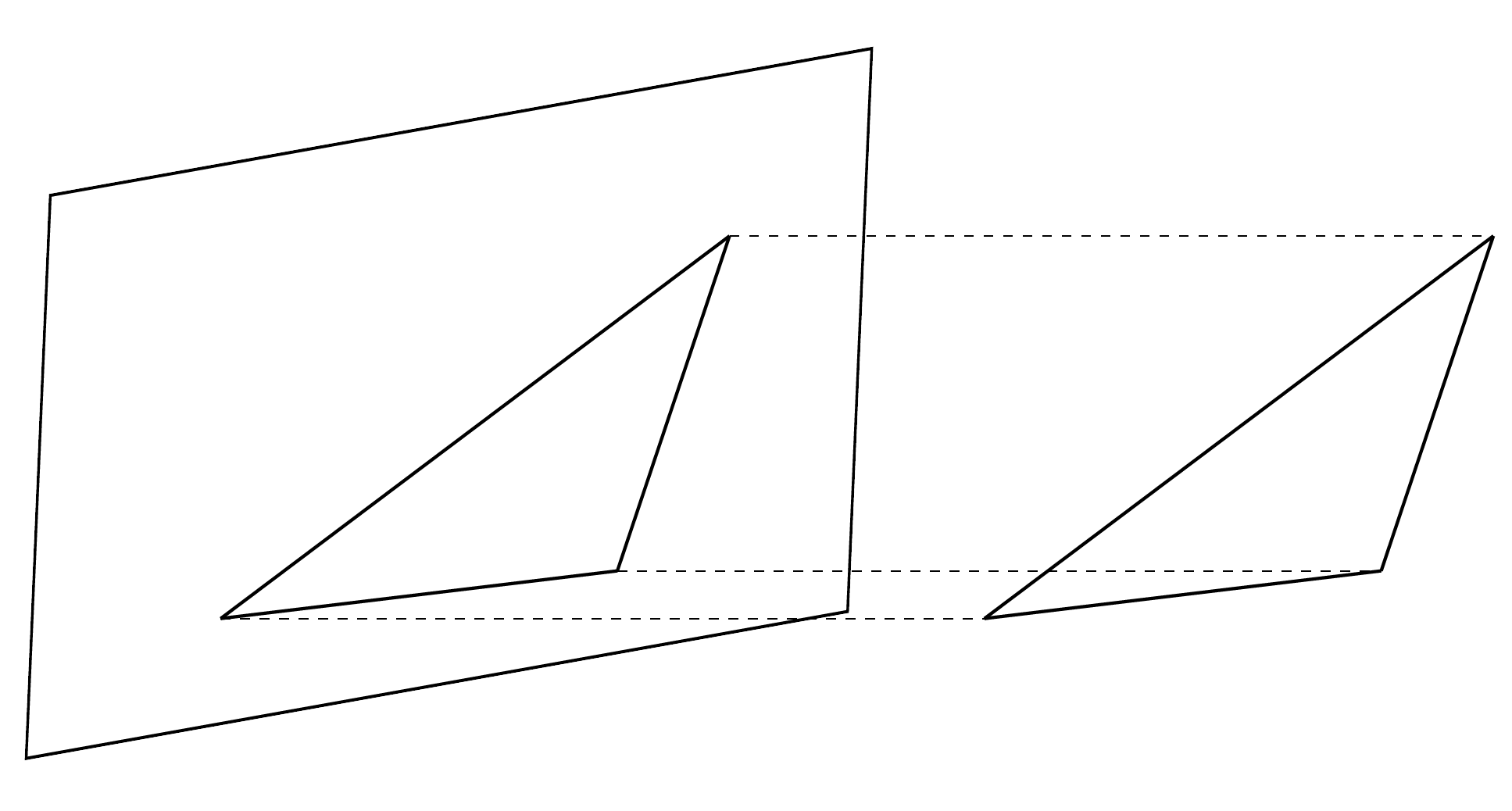
- A special case of perspective projection
- Center of projection (optical center) is at an infinite distance away from the image plane
$$ \left( \begin{array}{c} X \\ Y \\ 1 \end{array} \right) = \left[ \begin{array}{cccc} 1 & 0 & 0 & 0 \\ 0 & 1 & 0 & 0 \\ 0 & 0 & 0 & 1 \end{array} \right] \left( \begin{array}{c} X \\ Y \\ Z \\ 1 \end{array} \right) $$
Cameras exhibiting weak perspective
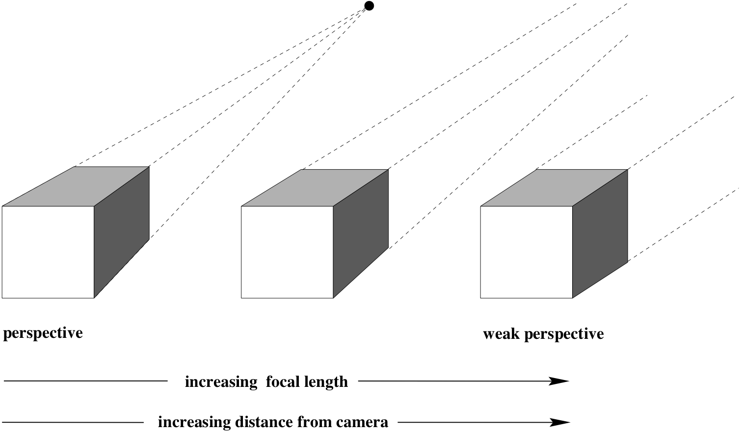
- Object dimensions are much smaller compared to its distance from the camera, e.g., satellite imagery
$$ \left( \begin{array}{c} x \\ y \\ \lambda \end{array} \right) = \left[ \begin{array}{cccc} 1 & 0 & 0 & 0 \\ 0 & 1 & 0 & 0 \\ 0 & 0 & 0 & \lambda \end{array} \right] \left( \begin{array}{c} X \\ Y \\ Z \\ 1 \end{array} \right) $$
Pushbroom cameras
Pushbroom cameras is an abstraction for the type of sensors often used in satellite imaging (SPOTS). Here camera is a linear sensor array that captures one row of image at each time. The full image is constructed by moving the camera. When sensor moves, the sensor plane sweeps out a region of space.
Let $\mathbf{X}$ be a point in space, and lets assume that camera matrix is $\mathtt{P}$. Suppose that $\mathtt{P} \mathbf{X} = (x, y, w)^T$. Then the corresponding inhomogeneous image point is $(x, y/w)$. This assumes that the camera motion is along $x$ direction of the image.
Projective Geometry (Lessons)
- Distant objects appear smaller.
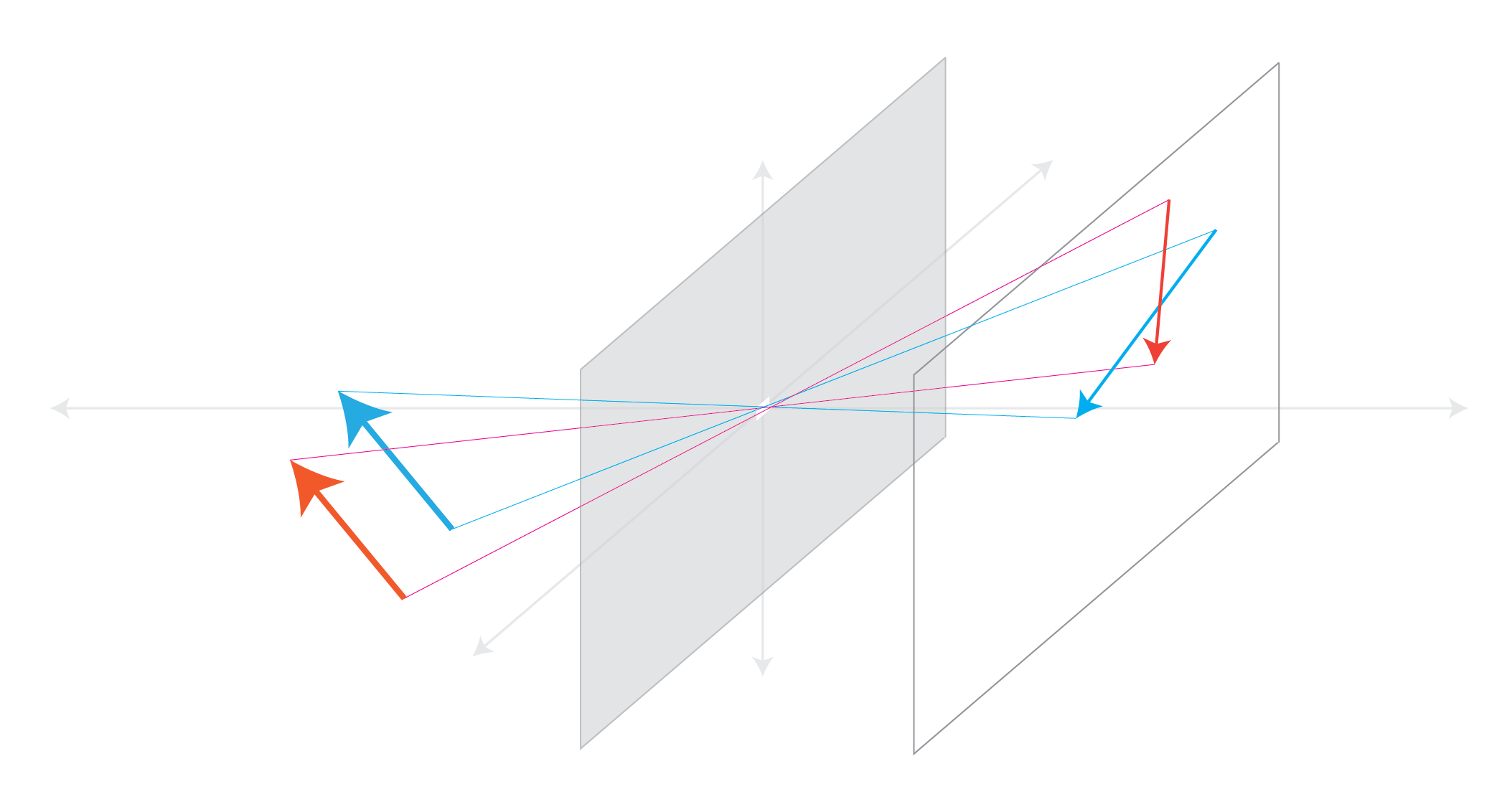
- The same object when imaged using different focal lengths appear to have different sizes.
- Parallel lines meet.
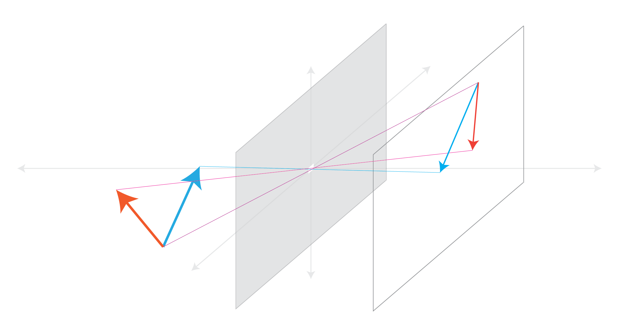
- Angles are not maintained, i.e., perpendicular lines appear meet at angles other than 90 degrees.
Distant Objects Appear Smaller
Focal Lengths
Angles are Not Preserved
Parallel Lines Meet
Vanishing Points
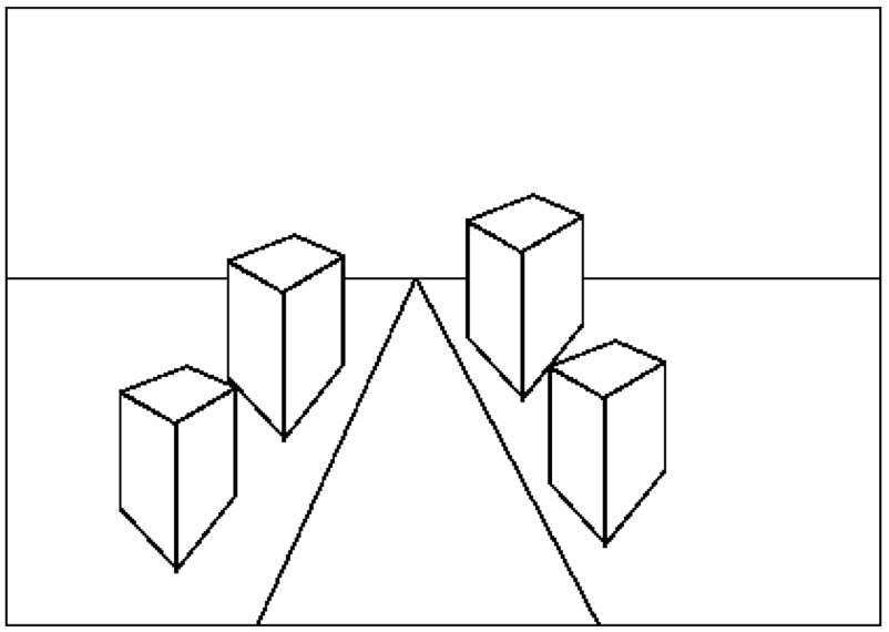
Each set of parallel lines meet at a different point on the image plane. This point is called the vanishing point for this direction.
Set of parallel lines in the same plane lead to *collinear vanishing points. The lines formed by these vanishing points is called that horizon for that plane.
Vanishing points can be used for 3D scene analysis
These can be used to spot fake images, e.g., scale or perspective doesn't work
Is this a perspective image of four identical buildings? If not, why not?
Lens Effects
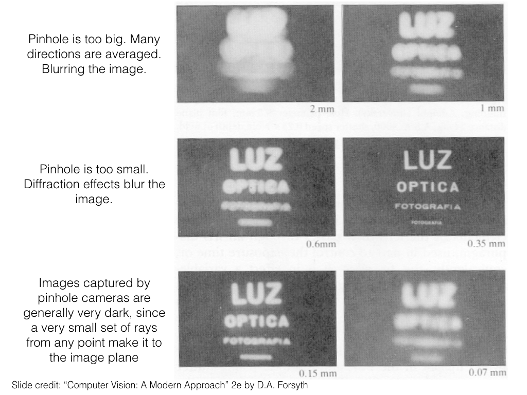
Images captured by pinhole cameras are generally two dark. In order to allow more light to pass through and reach the sensor plane, we need to increase the size of the pinhole. This has the effect of making the image blurry. We can undo this by using a lens that will focus the light onto the image plane. Lenses, however, introduce radial and chromatic distortions.
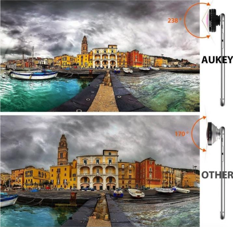
Modeling radial distortion to capture (and undo) lens effects
This discussion follows Ch. 7 of Multiple View Geometry in Computer Vision, Second Edition.
- $(\tilde{x}, \tilde{y})$ is the ideal image position (which obeys linear projection)
- $(x_d, y_d)$ is the actual image position (after radial distortion)
- $\tilde{r}$ is the radial distance $\sqrt{\tilde{x}^2 + \tilde{y}^2}$ from the center
- $L(\tilde{r})$ is the distortion factor (we make a simplifying assumption that the distorion is a function of radius only.
Then we can write
$$ \left( \begin{array}{c} x_d \\ y_d \end{array} \right) = L(\tilde{r}) \left( \begin{array}{c} \tilde{x} \\ \tilde{y} \end{array} \right) $$
Correction of distortion
In pixel coordinates, the correction is written as
$$ \begin{align} \hat{x} & = x_c + L(r) (x - x_c) \\ \hat{y} & = y_c + L(r) (y - y_c) \end{align} $$
Here $(x, y)$ are the measured coordinates, $(\hat{x},\hat{y})$ are the corrected coordinates, $(x_c, y_c)$ is the center of radial distorion, and $r = \sqrt{(x-x_c)^2 + (y-y_c)^2}$.
We often use Taylor expansion $L(r) = 1 + \kappa_1 r + \kappa_2 r^2 + \cdots$. The coefficient of radial distortions $\{\kappa_1, \kappa_2, x_c, y_c \}$ are considered part of the intrinsic matrix $\mathtt{K}$. These paramters are often estimated during camera calibration process. $L(r)$ can be estimated by minimizing the deviation from linear mapping, e.g., the distances of end-points of a line to its mid-point.
For further information, we refer the reader to Ch. 7 of Multiple View Geometry in Computer Vision (2nd Ed.) by Harley and Zisserman.
Camera calibration in OpenCV
Check out the camera-calibration notbook.
Appendix
Singular Value Decomposition
Consider an $m \times n$ matrix $\mathbf{M}$. SVD factorizes this matrix as follows:
$$ \mathbf{M} = \mathbf{U} \mathbf{\Sigma} \mathbf{V}^T, $$
where $\mathbf{U} \in \mathbb{R}^{m \times m}$, $\mathbf{\Sigma} \in \mathbb{R}^{m \times n}$, and $\mathbf{V} \in \mathbb{R}^{n \times n}$.
$\mathbf{\Sigma}$ is a rectangular diagonal matrix with non-negative real numbers on the diagonals. Diagonal entries $\sigma_i = \Sigma_{ii}$ are called singular values of $\mathbf{M}$. The number of non-zero singular values is equal to the rank of $\mathbf{M}$.
Columns of $\mathbf{U}$ form an orthonormal basis, i.e., $\mathbf{U}^T \mathbf{U} = \mathbf{I}$. Columns of $\mathbf{U}$ are also called left-singular vectors of $\mathbf{M}$.
Columns of $\mathbf{V}$ also form an orthonormal basis, i.e., $\mathbf{V}^T \mathbf{V} = \mathbf{I}$. Columns of $\mathbf{V}$ are similarly called right-singular vectors of $\mathbf{M}$.
If singular values are sorted from largest to smallest, we can re-write $\mathbf{M}$ as $$ \mathbf{M} = \sum_{i=1}^r \sigma_i \mathbf{u}_i \mathbf{v}_i^T, $$ where $r$ is refers to the rank of the matrix. Note also that $r \le \text{min}\{m,n \}$.
SVD is not unique.
Moore-Penrose Pseudo Inverse
Using SVD, we can compute Pseudo-Inverse $\mathbf{M}^+$ of $\mathbf{M}$ as follows
$$ \mathbf{M}^+ = \mathbf{V} \mathbf{\Sigma}^+ \mathbf{U}^T, $$
where $\mathbf{\Sigma}^+$ is constructed by taking the reciprocals of non-zero diagonal entries of $\mathbf{\Sigma}$. Additionally, if $\mathbf{M}$ is $m \times n$ then set $\mathbf{\Sigma}^+$ equal to $n \times m$. This is achieved by either appending $\mathbf{0}^T$ to get exactly $m$ rows or $\mathbf{0}$ to get exactly $n$ columns. $\mathbf{0}$ is a column-vector of $0$s of appropriate length.
Example
Compute pseudo-inverse of a matrix using SVD.
import numpy as np

M = np.array([[1,2,3,4],[2,4,8,0],[12,-8,-12,0]])
print('M (3x4):\n', M)
M (3x4):
 [[  1   2   3   4]
 [  2   4   8   0]
 [ 12  -8 -12   0]]
- Compute SVD
U, E, Vt = np.linalg.svd(M)
print('\nU (3x3):\n', U)
print('\nE (non-zero Sigma_ii in diag form):\n', E)
print('\nVt (4x4):\n', Vt)
U (3x3):
 [[-0.13334471 -0.47047655 -0.8722792 ]
 [-0.32814963 -0.8095341   0.48679806]
 [ 0.93516683 -0.35115005  0.04643961]]

E (non-zero Sigma_ii in diag form):
 [19.85439808  7.65819068  3.62698118]

Vt (4x4):
 [[ 0.52544318 -0.45635343 -0.71758575 -0.02686452]
 [-0.82308545 -0.17887896 -0.47973498 -0.2457377 ]
 [ 0.18158138 -0.04656298  0.19858707 -0.96198922]
 [-0.11605177 -0.87038828  0.46420708  0.11605177]]
- Check that we can use SVD to reconstruct the original matrix.
Reconstructed_M = np.zeros((3,4))

for i in range(len(E)):
    Reconstructed_M += ( E[i] * np.dot(U[:,i].reshape(3,1), Vt[i,:].reshape(1,4)) )

print('Reconstructed_M (3x4):\n', Reconstructed_M)
print('\nElement-wise squared reconstruction error (3x4):\n', (M - Reconstructed_M)**2)
Reconstructed_M (3x4):
 [[ 1.00000000e+00  2.00000000e+00  3.00000000e+00  4.00000000e+00]
 [ 2.00000000e+00  4.00000000e+00  8.00000000e+00  2.88657986e-15]
 [ 1.20000000e+01 -8.00000000e+00 -1.20000000e+01  2.22044605e-15]]

Element-wise squared reconstruction error (3x4):
 [[7.88860905e-31 3.15544362e-30 9.66354609e-30 7.88860905e-31]
 [1.26217745e-29 7.88860905e-31 1.26217745e-29 8.33234331e-30]
 [7.88860905e-29 1.26217745e-29 0.00000000e+00 4.93038066e-30]]
- Check U and V are orthonormal matrices.
print('U is orthonormal (U U^T):\n', np.dot(U, U.T))
print('\nV is orthonormal (V V^T):\n', np.dot(Vt, Vt.T))
U is orthonormal (U U^T):
 [[1.00000000e+00 1.66533454e-16 8.32667268e-17]
 [1.66533454e-16 1.00000000e+00 1.07552856e-16]
 [8.32667268e-17 1.07552856e-16 1.00000000e+00]]

V is orthonormal (V V^T):
 [[ 1.00000000e+00 -9.71445147e-17 -4.16333634e-17  2.77555756e-16]
 [-9.71445147e-17  1.00000000e+00 -5.55111512e-17 -2.77555756e-16]
 [-4.16333634e-17 -5.55111512e-17  1.00000000e+00  2.35922393e-16]
 [ 2.77555756e-16 -2.77555756e-16  2.35922393e-16  1.00000000e+00]]
- Compute $\mathbf{\Sigma}^+$
E_plus = np.diag( 1./E )
E_plus = np.vstack( (E_plus, np.zeros((1,3)) ) )
print('E_plus:\n', E_plus)
E_plus:
 [[0.05036667 0.         0.        ]
 [0.         0.13057915 0.        ]
 [0.         0.         0.27571138]
 [0.         0.         0.        ]]
- Compute $\mathbf{M}^+$
M_plus = np.dot(Vt.T, np.dot(E_plus, U.T))
print('M_plus (4x3):\n', M_plus)
M_plus (4x3):
 [[ 0.003367    0.1026936   0.06481481]
 [ 0.02525253  0.02020202 -0.01388889]
 [-0.01346801  0.08922559 -0.00925926]
 [ 0.246633   -0.1026936  -0.00231481]]
- Confirm $\mathbf{M} \mathbf{M}^+$ is an identity matrix.
print('M M_plus (should be an identity matrix):\n', np.dot(M, M_plus))
M M_plus (should be an identity matrix):
 [[ 1.00000000e+00  3.33066907e-16  2.18575158e-16]
 [-3.33066907e-16  1.00000000e+00  9.71445147e-17]
 [ 0.00000000e+00 -3.33066907e-16  1.00000000e+00]]
- Compute pseudo inverse using
numpy.linalg.pinv
print('Pseudo-inverse using pinv:\n',np.linalg.pinv(M))
Pseudo-inverse using pinv:
 [[ 0.003367    0.1026936   0.06481481]
 [ 0.02525253  0.02020202 -0.01388889]
 [-0.01346801  0.08922559 -0.00925926]
 [ 0.246633   -0.1026936  -0.00231481]]
Cross-Product
Cross-product of two vectors $(d,e,f)$ and $(r,s,t)$ is computed as seen below.
$$ \begin{align} (d,e,f) \times (r,s,t) &= \mathrm{det} \left[\begin{array}{ccc} \hat{i} & \hat{j} & \hat{k}\\ d & e & f \\ r & s & t \end{array} \right] \\ &=(et - sf) \hat{i} - (dt - rf) \hat{j} + (ds - re) \hat{k} \end{align} $$
