Scientific Libraries in Python

• A library is a set of reusable functions and objects
• Python has an extensive set of libraries for scientific computing:
  • IterTools: A library of iterator-related functions (e.g. combinations, permutations, Cartesian products)
  • NumPy: A library related to processing large-quantities of numbers
  • SciPy: A library of common math/science functions, such as calculating integrals, Fourier transforms, matrix operations, interpolation
  • SimPy: A library of symbolic programming functions and objects (e.g. algebra, calculus solvers)
  • MatPlotLib: A library of functions for plotting data in various ways

NumPy

• NumPy is a library for processing numeric data
• One of NumPy's most used features is its array class
  • NumPy arrays serve a similar function to lists in Python, but are a bit more intuitive, have more features, and are more efficient
  • Arrays in NumPy can be n-dimensional

import numpy as np

array1D = np.array([1,2,3,4,5])
print(array1D[0])

array2D = np.array([[1,2,3,4,5],[6,7,8,9,10]])
print(array2D[2,3])
                        

NumPy

• To create a 4x5 array/matrix of zeroes or random values

zeroMatrix = zeros((4,5))  # note the double brackets
randomMatrix1 = random.random((4,5)) # range: [0,1]
                        

NumPy

• To create an array from a range
  • Similar to range() for lists, except that decimal steps are possible:

digits = np.arange(0, 10, 1)
evens = np.arange(0, 100, 2)
byHalf = np.arange(0, 10, 0.5)
                        

• To create an array containing a specified number of values between a maximum and minimum:

list = np.linspace(0, 10, 50)       # 50 data points
xCoords = np.linspace(0, 2*pi, 100) # 100 data points
                        

NumPy

• Scalar arithmetic operations are applied to all elements in a list:

xCoords = np.linspace(0, 2 * np.pi, 100)
yCoords = np.sin(xCoords)
print(np.array([1,2,3]) * 2)   # [2,4,6]
                        

NumPy

• Some useful functions:

matrix = np.array([[1,2,3],[7,9,8],[6,5,4]])
print(matrix.min())    # 1
print(matrix.max())    # 9
print(matrix.sum())    # 45
                        

• You can also do this for rows or columns:

matrix = np.array([[1,2,3],[7,9,8],[6,5,4]])
print(matrix.min(axis=0))   # column minimum:     [1,2,3]
print(matrix.max(axis=1))   # row maximum:        [3,9,6]
print(matrix.sum(axis=1))   # row sum:            [6,24,15]
                        

NumPy

• Iterating over rows in a matrix:

matrix = np.array([[1,2,3],[7,9,8],[6,5,4]])
for row in matrix:
   print(row)
                        

NumPy

• To reorder elements in a random order:

list = [1,2,3,4,5,6,7,8,9]
np.random.shuffle(list)
print('Shuffled:', list)
                        

NumPy

• To solve the following quadratic equations:
  • 2x⁰ + 4x¹ + 3x² = 5
  • 1x⁰ + 5x¹ + 1x² = 8
  • 3x⁰ + 2x¹ + 2x² = 4

coeff = np.array([[2,4,3],
                  [1,5,1],
                  [3,2,2]])
vals = np.array([5,8,4])
print('Solutions:', np.linalg.solve(coeff, vals))
# [1.05263158 1.63157895 -1.21052632]
                        

• For more linear algebra-related functions, check out:
  • http://docs.scipy.org/doc/numpy/reference/routines.linalg.html
  • http://docs.scipy.org/doc/scipy/reference/tutorial/linalg.html

NumPy

• To load an array from a file:

vals = np.loadtxt(fname='data1.csv', delimiter=',')
print(vals)
# [[1,2,3],
#  [4,5,6],
#  [7,8,9]]
                        

• To load an array of strings and other types from a file:

data = np.genfromtxt('data2.csv', dtype=None, delimiter=",")
print(vals)
# [[1, 2, 224690, 5.97222057420059, 'K3V', 0.999]
#  [2, 3, 224699, -1.1464684004746, 'B9', -0.019]]
                        

NumPy

• To save an array to a file:

array = np.array([[1,2,3,4],
                  [5,6,7,8],
                  [9,10,11,12],
                  [13,14,15,16]])
np.savetxt(fname='data.txt', delimiter=',', X=array)
                        

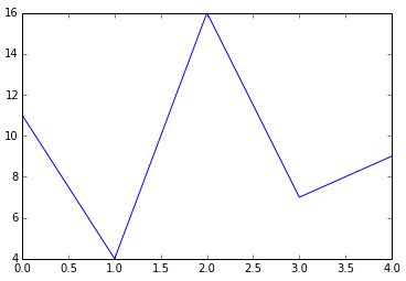
Line Plots: X-values Only

• To plot a set of numbers as y values:

import matplotlib.pyplot as plt
plt.plot([11,4,16,7,9])
plt.show()
                        

Line Plots: X and Y Values

• To plot a set of (x,y) values:

import matplotlib.pyplot as plt
plt.plot([1,2,3,4,5], [8,2,4,11,6], "r--")
plt.show()
                        

Line Plots: Multi-series

• To plot multiple series of data:

import matplotlib.pyplot as plt
plt.plot([1,2,3,4,5], [11,4,16,7,9], "r--",
         [1,2,3,4,5], [8,2,4,11,6],  "b-")
plt.show()
                        

All Plots: Labels

• To set the various labels:

plot = plt.plot([1,2,3,4,5], [8,2,4,11,6], "r--")
plt.xlabel('Week')
plt.ylabel('Score')
plt.title('Performance')
plt.show()
                        

All Plots: Axes

• To configure the ranges of the axes:
  • Minimum X, Maximum X, Minimum Y, Maximum Y

plot = plt.plot([1,2,3,4,5], [8,2,4,11,6], "r--")
plt.axis([1, 5, 0, 15])
plt.grid(True)
plt.show()
                        

All Plots: Logarithmic Scale Axes

• To configure the axes to use a logarithmic scale:

plot = plt.plot([1,10,100,1000,10000], [81,208,4120,117,6246], "r--")
plt.semilogx()
plt.semilogy()
plt.grid(True)
plt.show()
                        

Line Plots: Customized Appearance

• Line style:
  • '-' – solid line
  • '--' – dashed line
  • '-.' – dot-dashed combination
  • ':' – dotted line
  • 'steps' – draw horizontal lines between points

Line and Scatter Plots: Customized Appearance

• Point marker:
  • '+' – plus sign
  • '.' - dot
  • 's' - square
  • 'o' - circle
  • '^' – triangle

All Plots: Customized Appearance

• Colour:
  • 'r' – read
  • 'b' – blue
  • 'g' – green
  • 'c' – cyan
  • 'm' – magenta
  • 'y' – yellow
  • 'k' – black
  • 'w' - white

Line Plots: Functions

• To plot functions:

import matplotlib.pyplot as plt
xs = np.arange(0.0, 4.0, 0.2)
plt.plot(xs, xs**2, 'bo',
         xs, xs**3, 'gs',
         xs, xs**4, 'r^')
plt.show()
                        

Line Plots: Customized Appearance

• Using line styles:

import matplotlib.pyplot as plt
plot = plt.plot([1,2,3,4,5], [8,2,4,11,6], "r--")
plt.setp(plot, linestyle='-.', marker='+',
               linewidth='2.0', color='b')
plt.show()
                        

Line Plots: Customized Appearance

• Figure size:

plot = plt.plot([1,2,3,4,5], [8,2,4,11,6], "r--")
figure = plt.gcf()  # get current figure
figure.set_size_inches(8.0, 5.0)
                        

Line Plots: Exporting as an Image

• Saving a plot, as an image file:

plot = plt.plot([1,2,3,4,5], [8,2,4,11,6], "r--")
figure = plt.gcf()  # get current figure
figure.set_size_inches(8.0, 5.0)
figure.savefig('test_results.png', dpi=100)
                        

Histograms

• To draw a histogram (bar chart of frequencies):

x = 60 + 15 * np.random.randn(10000)
numBuckets = 50
plt.hist(x, numBuckets, normed=1, facecolor='b')
plt.xlabel('Grade')
plt.ylabel('Probability')
plt.axis([0, 100, 0, 0.05])
plt.grid(True)
plt.show()
                        

Bar Charts

• To draw a bar chart:

indices = np.arange(5)
spending = [17000, 21500, 10500, 9800, 16000]
earnings = [28000, 20350, 11300, 12000, 14500]
width = 0.3
p1 = plt.bar(indices, spending, width, color='b')
p2 = plt.bar(indices+width, earnings, width, color='r')
plt.show()
                        

All Charts: Legend

• To show a legend:

p1 = plt.bar(indices, spending, width, color='b')
p2 = plt.bar(indices+width, earnings, width, color='r')
plt.legend((p1[0],p2[0]), ('Spending','Earnings'))
plt.show()
                        

Pie Charts

• To show a pie chart:

labels = 'Biology','Forensics','Chemistry','Comm. Studies'
counts = [81, 92, 41, 17]
clrs = ['gold','yellowgreen','lightcoral','lightskyblue']
expl = (0, 0, 0.1, 0)
plt.pie(counts, explode=expl, labels=labels, colors=clrs,
autopct='%1.1f%%', shadow=True, startangle=90)
plt.axis('equal')
plt.show()
                        

Wireframe Plots

import scipy.misc as misc
from mpl_toolkits.mplot3d import Axes3D
Z = misc.ascent()
X = np.arange(0, Z.shape[0], 1)
Y = np.arange(0, Z.shape[1], 1)
X, Y = np.meshgrid(X, Y)
fig = plt.figure()
ax = fig.gca(projection='3d')
ax.plot_wireframe(X, Y, Z, rstride=10, cstride=10)
plt.show()
                        

Surface Plots

import scipy.misc as misc
from mpl_toolkits.mplot3d import Axes3D
from matplotlib import cm
Z = misc.ascent()
X = np.arange(0, Z.shape[0], 1)
Y = np.arange(0, Z.shape[1], 1)
X, Y = np.meshgrid(X, Y)
fig = plt.figure()
ax = fig.gca(projection='3d')
surf = ax.plot_surface(X, Y, Z, rstride=1, cstride=1,
                 cmap=cm.coolwarm, linewidth=0, antialiased=False)
plt.show()
                        

Contour Plots

fig = plt.figure()
ax = fig.gca(projection='3d')
X, Y, Z = axes3d.get_test_data(0.05)
ax.plot_surface(X, Y, Z, rstride=8, cstride=8, alpha=0.3)
cset = ax.contourf(X, Y, Z, zdir='z', offset=-100, cmap=cm.coolwarm)
cset = ax.contourf(X, Y, Z, zdir='x', offset=-40, cmap=cm.coolwarm)
cset = ax.contourf(X, Y, Z, zdir='y', offset=40, cmap=cm.coolwarm)
ax.set_xlim(-40, 40)
ax.set_ylim(-40, 40)
ax.set_zlim(-100, 100)
plt.show()
                        

Scatter Plots

def randrange(n, vmin, vmax):
   return (vmax-vmin)*np.random.rand(n) + vmin
fig = plt.figure()
ax = fig.add_subplot(111, projection='3d')
n = 100
for c, m, zl, zh in [('r', 'o', -50, -25), ('b', '^', -30, -5)]:
   xs = randrange(n, 23, 32)
   ys = randrange(n, 0, 100)
   zs = randrange(n, zl, zh)
   ax.scatter(xs, ys, zs, c=c, marker=m)
plt.show()